Your catalog was built for people to find. Now AI has to understand it.
Most publishers hold thousands, often millions, of PDFs, laid down in layers over thirty years. Each layer solved the problem of its day.
1990s
You went digital
The paper archive was scanned into PDFs, one picture per page. The pages survived. What was on them, to software, did not.
Old or new, your PDFs weren't made for AI.
A scan from 1960 and a PDF from last month fail in different ways, but both fail. Getting your corpus ready means more than better OCR: every page has to be rebuilt as a document an AI can navigate, quote, and credit. That is what Cashmere does, for every PDF you hold.
The problem
Not all PDFs are created equal
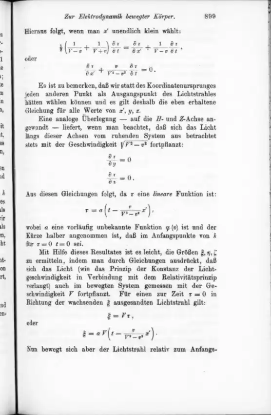
Whether software can read a PDF depends on how it was made, and the oldest files, often the most valuable in a catalog, are the hardest of all. Here is one equation from each kind, three ways.
1
Hard
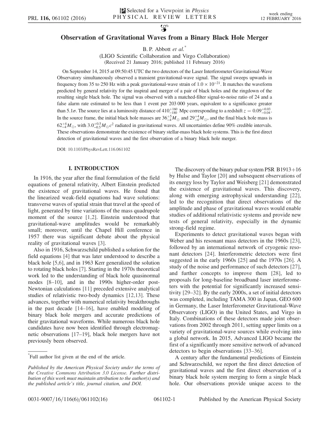
Born digital
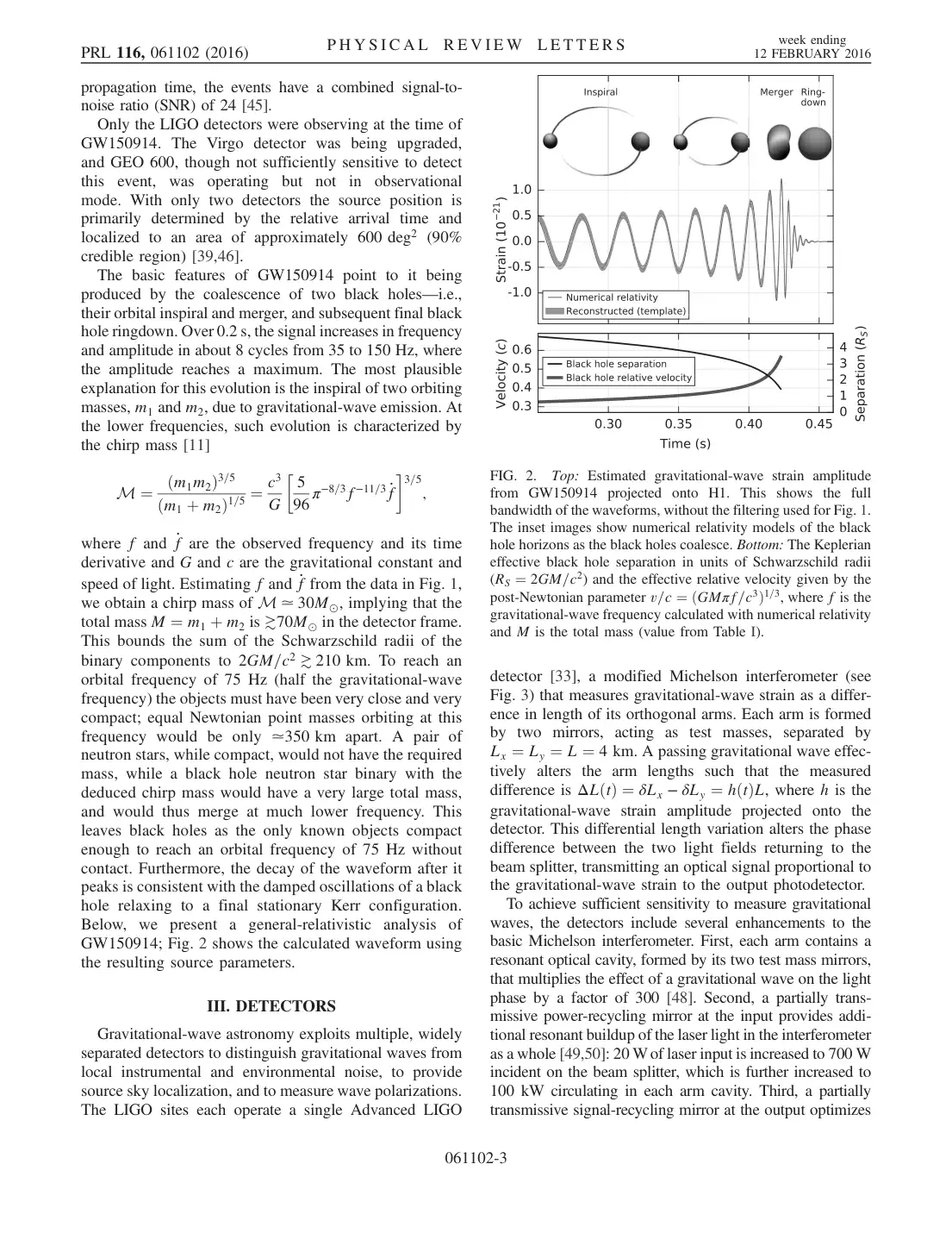
LIGO 2016 · Kakeya 2025 · Beilstein 2026
The text is real, but it is stored as letters placed on a page, in the font’s own private encoding. Fractions fall apart, = becomes ¼, and a two-column page reads straight across both columns.
The page
What the PDF's own text says
M ¼ ðm1m2Þ3=5 ðm1 þ m2Þ1=5 ¼ c3 G 5 96 π−8=3f−11=3 _f 3=5 ;
A photograph of a printed page. The only text is an OCR layer added later, which reads ordinary words and gives up on everything else: equations, tables, and symbols.
The page
What the PDF's own text says
=
Ot
Or
9:
oder
let.
OCR layer: fragments
What the omnipub says
21(V−v1+V+v1)∂t∂τ=∂x′∂τ+V−v1∂t∂τ,
∂x′∂τ+V2−v2v∂t∂τ=0.
Einstein, 1905, page 9
3
Hardest
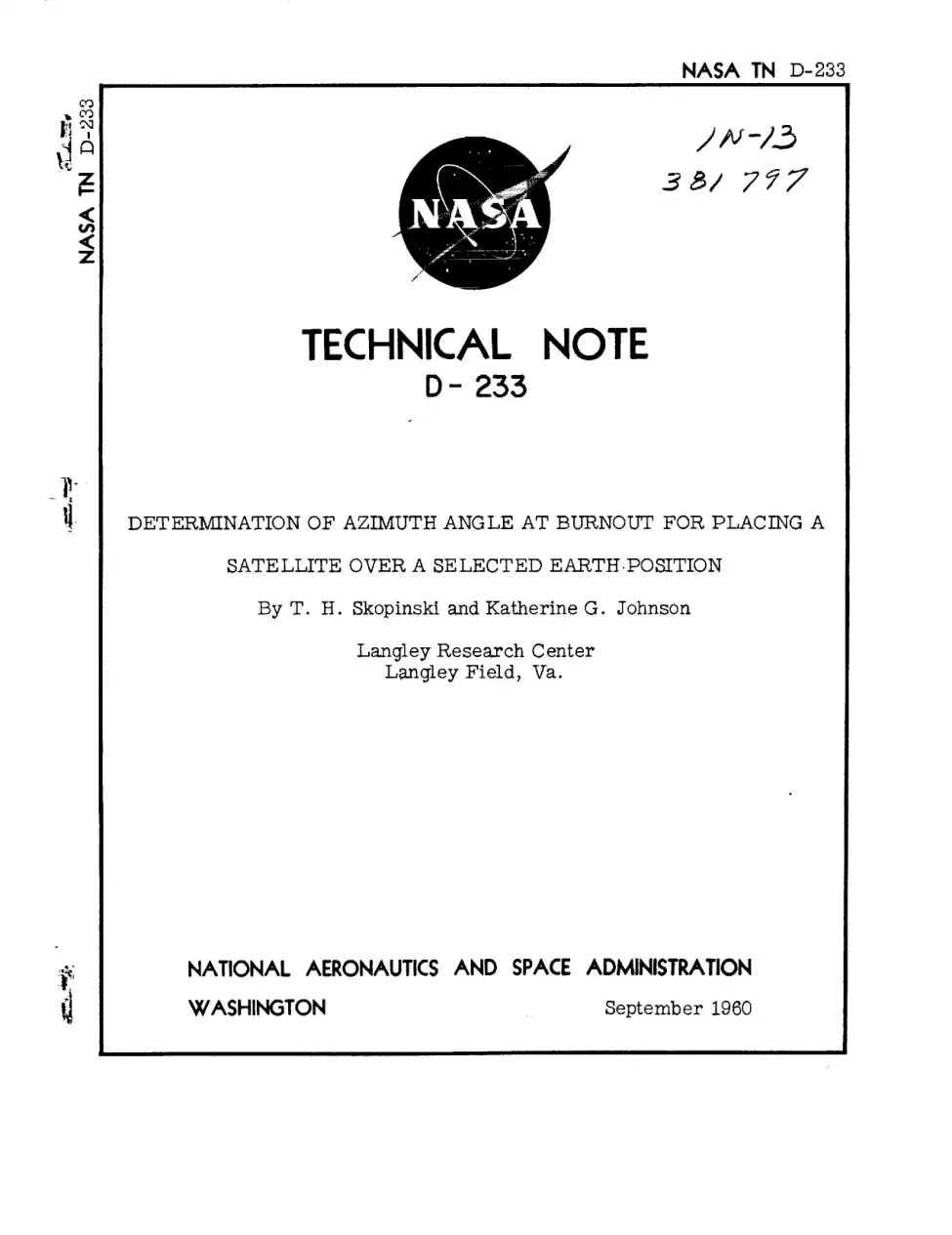
Typewritten originals
NASA TN D-233, Katherine Johnson, 1960
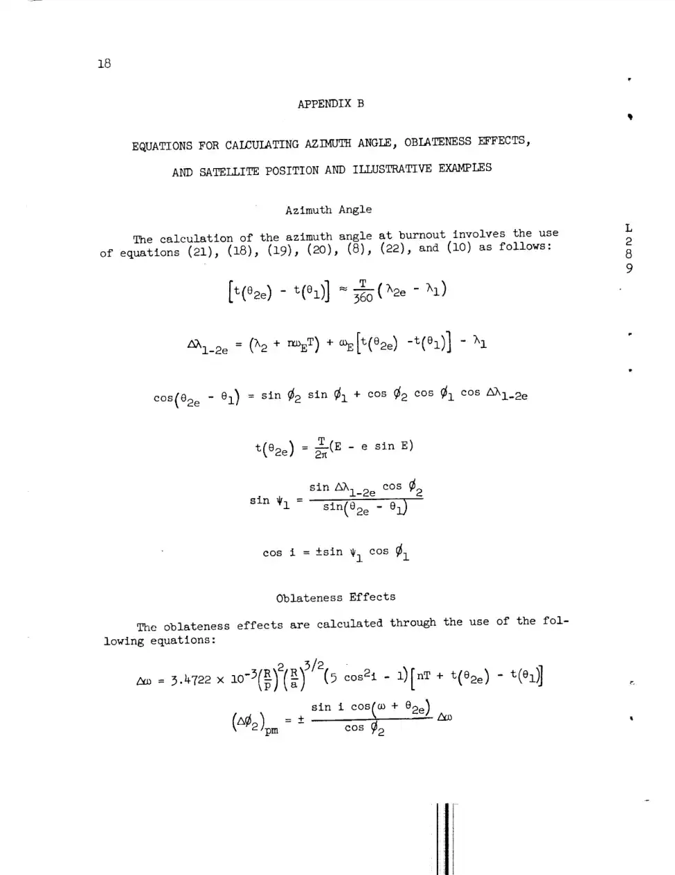
Typed, copied, and scanned from the copy. Uneven strikes, stamps, and margin notes, and Greek letters the OCR never learned: every λ, ω, and θ below is lost or misread.
The page
What the PDF's own text says
2_i_2e = (h2 + r_oET) + _E[t(e2e) -t(el)] - h I
OCR layer: symbols lost
What the omnipub says
Δλ1−2e=(λ2+nωET)+ωE[t(θ2e)−t(θ1)]−λ1
NASA TN D-233, 1960, page 20
Why it matters
AI can only use what it can read.
A paper that fails ingestion is invisible: it can’t be searched, retrieved, cited, or licensed.
Wrong is worse than missing.
A misread number in a table or a garbled equation doesn’t look broken to an AI. It gets quoted, confidently.
The back catalog is the hard part.
Decades of scanned journals, reports, and books hold a publisher’s most distinctive content, and they are the nastiest PDFs of all.
How it works
From a page of ink to a document AI can use
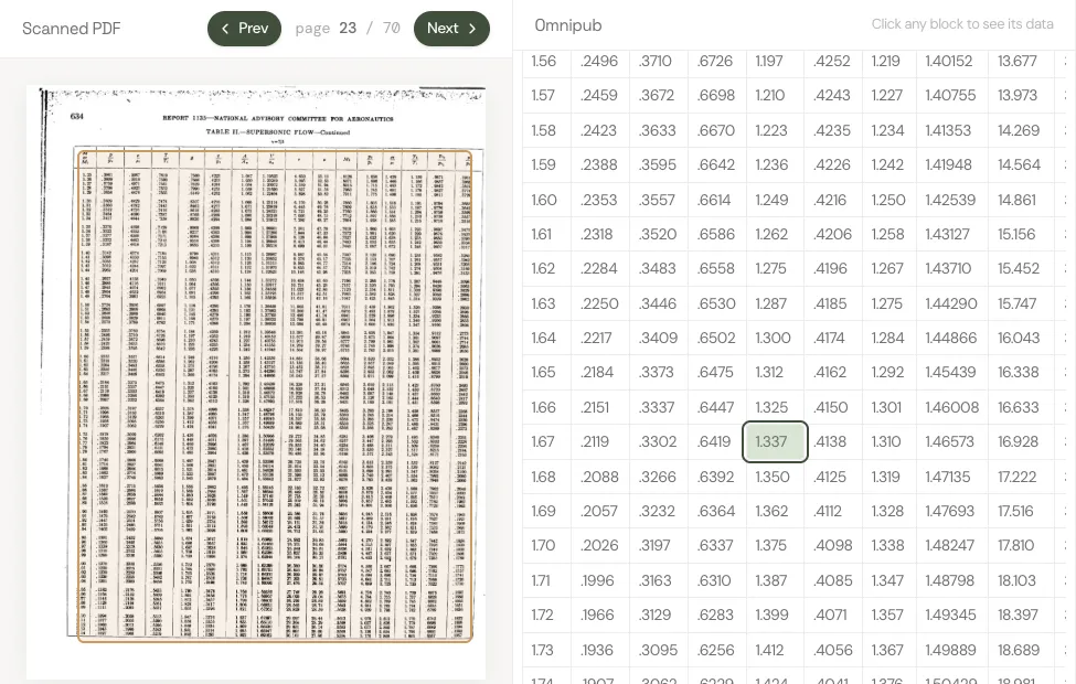
One page of Katherine Johnson’s 1960 NASA paper, all the way through Cashmere. Every picture below is the real page and the real output.
STEP 01
Start with a PDF
A PDF records where ink goes on a page. To software, this page is a picture: the equations aren't text at all, and its OCR layer reads them as noise.
STEP 02
Read the page like a person
The Pro parser finds the structure a reader sees: which marks are a heading, a paragraph, an equation, a table, or a figure, and the order they're read in.
heading26
paragraph235
equation84
table11
figure13
list item24
787 blocks in the whole paper
STEP 03
Make every piece a block
Each piece becomes an omnipub block with a type and a stable address, so it can be searched, quoted, cited, and licensed on its own. Equations become real math.
Contents
SUMMARY3
INTRODUCTION4
SYMBOLS102
SATELLITE POSITION RELATIONSHIPS5
EXPRESSION FOR PLACING A SATELLITE OVER A SELECTEDPOSITION27
APPENDIX B1
EQUATIONS FOR CALCULATING AZIMUTH ANGLE, OBLATENESS EFFECTS,AND SATELLITE POSITION AND ILLUSTRATIVE EXAMPLES1
The blocks are put back together as the paper itself: sections inside sections, in reading order, each with its own address. The result is one document an AI can navigate and measure, from its table of contents down to a single equation.
Every block remembers where it sat on the original page. An answer can cite the exact equation it used, and anyone can check it against the source.
Pick a paper below to see every page and every block side by side.
Why Cashmere
Parsed isn’t the same as AI-ready
Plenty of tools can pull text out of a PDF. An AI needs more: what each piece is, where it belongs, where it came from, and what it may be used for. That is the work Cashmere does, on the files other pipelines give up on.
Right on the hard pages
Layout, text, math, and tables are read from the page image itself, not from the broken text layer, so a 1905 scan comes out as clean as a 2025 preprint.
Structured like the work
Headings, sections, and reading order are kept, and every block gets a stable address. An AI can find the right passage instead of guessing from a wall of text.
Traceable to the source
Every block keeps its place on the original page. An answer can cite the exact paragraph or equation it used, and anyone can check it.
Licensed and measured
Rights travel with the content, and use is counted block by block, so you know what AI systems read and you get paid for it.
6 papers, 335 pages, from a 1905 scan to a 2025 preprint, converted by one pipeline with no hand corrections. Bring us your hardest PDFs.
Converted by Cashmere’s Pro parser, November 2026, and shown without hand corrections.
Thousands of PDFs or millions, ready for AI.
Cashmere converts your entire corpus quickly and accurately, from decades-old scans to last month’s releases, so AI can read it, cite it, and credit you.
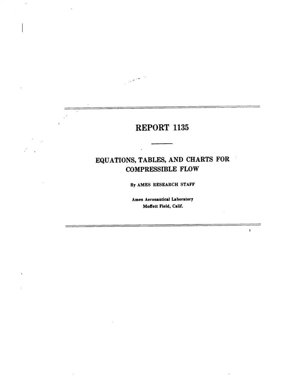
EQUATIONS, TABLES, AND CHARTS FOR COMPRESSIBLE FLOW 1
By AMES RESEARCH STAFF
SUMMARY
This report, which is a revision and extension of NACA TN 1428, presents a compilation of equations, tables, and charts useful in the analysis of high-speed flow of a compressible fluid. The equations provide relations for continuous one-dimensional flow, normal and oblique shock waves, and Prandtl-Meyer expansions for both perfect and imperfect gases. The tables present useful dimensionless ratios for continuous one-dimensional flow and for normal shock waves as functions of Mach number for air considered as a perfect gas. One series of charts presents the characteristics of the flow of air (considered a perfect gas) for oblique shock waves and for cones in a supersonic air stream. A second series shows the effects of caloric imperfections on continuous one-dimensional flow and on the flow through normal and oblique shock waves.
INTRODUCTION
The practical analysis of compressible flow involves frequent application of a few basic results. A convenient compilation of equations, tables, and charts embodying these results is therefore of great assistance in both research and design. The present report makes one of the first such compilations (ref. 1) more readily available in a revised and extended form. The revisions include a complete rewriting of the lists of equations, as well as the correction of certain typographical errors which appeared in the earlier work. The extensions are primarily in the directions dictated by increasing flight speeds, that is, to higher Mach numbers and to higher temperatures with the accompanying gaseous imperfections.
Compilations similar to those of reference 1 have been given in other publications, as, for example, references 2 through 6. These references have been utilized in extending the tables and charts to higher values of the Mach number. The extension to imperfect gases is based on the relations presented in references 7 and 8.
SYMBOLS AND NOTATION
PRIMARY SYMBOLS
a
speed of sound
A
cross-sectional area of stream tube or channel
CN
normal-force coefficient for cones, q∞Sbnormal force
cp
specific heat at constant pressure
cv
specific heat at constant volume
h
enthalpy per unit mass, u+pv
l
characteristic reference length
M
Mach number, aV
p
pressure 2
q
dynamic pressure, ρV2/2
q
heat added per unit mass
R
gas constant
R
Reynolds number, μρVl
Sb
base area of cone
s
entropy per unit mass
T
absolute temperature 2
u
internal energy per unit mass
v
specific volume, ρ1
u,v
velocity components parallel and perpendicular respectively, to free-stream flow direction
u~,v~
velocity components normal and tangential, respectively, to oblique shock wave
V
speed of flow
Vm
maximum speed obtainable by expanding to zero absolute temperature
w
external work performed per unit mass
α
angle of attack
β
M2−1
γ
ratio of specific heats, cvcp
δ
angle of flow deflection across an oblique shock wave
θ
shock-wave angle measured from upstream flow direction
Θ
molecular vibrational-energy constant
μ
Mach angle, sin−1M1
μ
absolute viscosity
ν
Prandtl-Meyer angle (angle through which a supersonic stream is turned to expand from M=1 to M>1)
1 Supersedes NACA TN 1428, "Notes and Tables for Use in the Analysis of Supersonic Flow" by the Staff of the Ames 1- by 3-foot Supersonic Wind-Tunnel Section, 1947.
2 When used without subscripts, p, ρ, and T denote static pressure, static density, and static temperature, respectively.
ξ
pressure ratio across a shock wave, p1p2
ρ
mass density2
σ
semivertex angle of cone
SUBSCRIPTS
∞
free-stream conditions
1
conditions just upstream of a shock wave
2
conditions just downstream of a shock wave
t
total conditions (i. e., conditions that would exist if the gas were brought to rest isentropically)
*
critical conditions (i. e., conditions where the local speed is equal to the local speed of sound)
c
conditions on the surface of a cone
r
reference (or datum) values
perf
quantity evaluated for a gas which is both thermally and calorically perfect
therm perf
quantity evaluated for a gas which is thermally perfect but calorically imperfect
( )p
derivative evaluated at constant pressure
( )s
derivative evaluated at constant entropy
( )T
derivative evaluated at constant temperature
( )v
derivative evaluated at constant specific volume
( )rev
quantity evaluated over a reversible path
NOTATION
The notation in brackets [ ] after many of the equations signifies that the equation is valid only within certain limitations. For example:
[perf] means that the equation is restricted to a gas which is both thermally and calorically perfect. (By "thermally perfect" it is meant that the gas obeys the thermal equation of state p=ρRT. By "calorically perfect" it is meant that the specific heats cp and cv are constant.)
[therm perf] means that the only restriction on the gas is that it must be thermally perfect. Equations so marked may be used for calorically imperfect gases. (They are, of course, also valid for completely perfect gases.)
[isen] means that the flow process must take place isentropically. Equations so marked may not be applied to the flow across a shock wave.
[adiab] means that the only restriction on the flow process is that it must take place adiabatically—that is, without heat transfer. (Such a flow process may or may not be isentropic depending on whether it is or is not reversible.) Equations so marked may be applied to the flow across a shock wave.
An equation without notation has no restrictions beyond those basic to the study of thermodynamics and/or inviscid compressible flow.
FUNDAMENTAL RELATIONS
THERMODYNAMICS
THERMAL EQUATIONS OF STATE
A thermal equation of state is an equation of the form
p=p(v,T)(1)
Several of the more commonly used thermal equations of state are the following:
Equation for thermally perfect gas
p=vRT=ρRT [therm perf](2)
or
pdp−ρdρ−TdT=0 [therm perf](3)
Equations for thermally imperfect gas
Van der Waals' equation (ref. 9)
p=v−bRT−v2a(4)
where a is the intermolecular-force constant and b is the molecular-size constant (see ref. 9, pp. 390 et seq. for numerical values).
Berthelot's equation (ref. 7)
p=v−bRT−v2Tc(5)
where b is the molecular-size constant and c is the intermolecular-force constant (see ref. 7 for numerical values).
Beattie-Bridgeman equation (ref. 10)
p=v2RT(1−vT3c)[v+B0(1−vb)]−v2A0(1−va)(6)
where a, A0, b, B0, and c are constants for a given gas (see ref. 10, p. 270 for numerical values).
CALORIC EQUATION OF STATE
A caloric equation of state is an equation of the form
On the basis of the above results, useful relations can be derived expressing various dimensionless ratios as functions of a single parameter. These relations are given below, grouped according to which of the various parameters (M, V/a∗, V/at, or V/Vm) is used as the independent variable.
In each case the second form of the equation applies for γ=57.
Tables I and II list numerical values of the following ratios with Mach number M as the independent variable:
ptp,ρtρ,TtT,ptq,a∗V
STREAM-TUBE-AREA RELATIONS
If it is assumed that the density and speed are uniform across any section of a given stream tube, then the equation of continuity is
ρVA=constant=ρ∗a∗A∗(79)
By combining this and certain of the foregoing equations, the area ratio A∗/A can be expressed as a function of any one of the four parameters used above. The final equations are
Numerical values of A∗/A as a function of M are given in tables I and II.
Equation (79) combined with equations (26), (29b), (45), and (46) can be employed to obtain the mass-flow rate per unit area ρV along a stream tube as a function of Mach number, total temperature, and total pressure. Numerical values can be obtained conveniently from chart 1 where the variation with Mach number of the mass-flow rate per unit cross-sectional area is presented for various total temperatures and a total pressure of 1 pound per square inch absolute.
SHOCK WAVES
NORMAL SHOCK WAVES
BASIC EQUATIONS
The previous relations for isentropic flow are valid on either side of a shock wave, but not across it, because at the shock wave the flow quantities have discontinuities. Jump
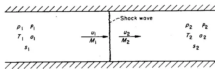
A diagram of a 1D channel bounded by two horizontal walls. A vertical line represents a shock wave. On the left (upstream), the state is p1,p1,T1,o1,s1 with velocity u1 and mass flux M1. On the right (downstream), the state is p2,p2,T2,o2,s2 with velocity u2 and mass flux M2. Arrows indicate the flow direction from left to right.
Shock wave
p1
p1
u1
M1
p2
p2
T1
o1
T2
o2
s1
s2
Scientific illustration: One-dimensional flow with a shock wave between two states.
FIGURE 1.—Notation for normal shock wave.
conditions for a steady normal shock wave (fig. 1) result from requiring conservation of
together with the requirement that the entropy does not decrease:
Δs≡s2−s1≥0(87)
It follows immediately from the energy relation (86) that total enthalpy, total temperature, and total speed of sound are constant across the shock and hence (from the previous relations (33) for adiabatic flow) also the critical speed of sound and limiting speed:
Combining equations (84) to (86) leads to Prandtl's relation
u1u2=a∗2=ρ2−ρ1p2−p1[adiab, perf](89)
which implies that the flow is supersonic ahead of the shock wave and subsonic behind (the reverse possibility is ruled out by the requirement of nondecreasing entropy), and to the Rankine-Hugoniot relations
Many relations for normal shock waves are conveniently expressed in terms of either upstream Mach number M1 or the static-pressure ratio across the shock ξ≡p2/p1. The following relations apply to adiabatic flow of a completely perfect fluid. The last form of each equation holds for γ=7/5.
In unsteady flow a normal shock wave acts at each instant as a steady shock. Hence all the above relations are valid across a moving normal shock wave if instantaneous velocities are measured relative to the shock.
OBLIQUE SHOCK WAVES
In general, a three-dimensional shock wave will be curved, and will separate two regions of nonuniform flow. However, the shock transition at each point takes place instantaneously, so that it is sufficient to consider an arbitrarily small neighborhood of the point. In such a neighborhood
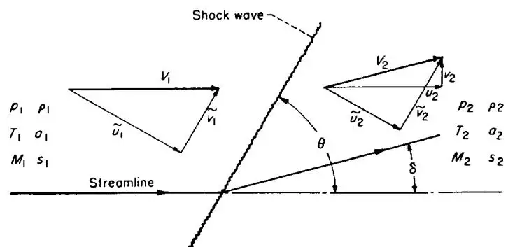
A diagram illustrating the flow properties across a shock wave. On the left, upstream of the shock, a velocity triangle is shown with velocity components V1, u~1, and v~1. The thermodynamic states p1, ρ1, T1, a1, and M1, s1 are listed. On the right, downstream of the shock, another velocity triangle is shown with components V2, u~2, and v~2. The thermodynamic states p2, ρ2, T2, a2, and M2, s2 are listed. The shock wave is inclined at an angle θ to the streamline. The angle δ is shown between the streamline and the downstream flow direction.
Shock wave
V1
p1ρ1
T1a1
M1s1
Streamline
θ
δ
V2
p2ρ2
T2a2
M2s2
Scientific illustration: Velocity triangles and thermodynamic states across a shock wave.
FIGURE 2.—Notation for oblique shock wave.
the shock wave may be regarded as plane to any desired degree of accuracy, and the flows on either side as uniform and parallel. Moreover, with the proper orientation of axes the flow is locally two-dimensional. Hence it is sufficient to consider a straight oblique shock wave in a uniform parallel two-dimensional stream, as shown in figure 2.
BASIC EQUATIONS
For a steady oblique shock wave, jump conditions result from requiring conservation of
together with the requirement that the entropy does not decrease:
Δs=s2−s1≥0(119)
Again it follows from the energy relation (118) that total enthalpy, total temperature, and total speed of sound are constant across the shock and hence also the critical speed of sound and limiting speed:
* Compare remark for normal shock waves, footnote on page 618.
CONNECTION WITH NORMAL SHOCK
A comparison of equation (115) with (117) shows that the tangential velocity is constant across the shock wave:
v~1=v~2[adiab](122)
so that the change in velocity is normal to the shock. It follows that
21v~12=21v~22
so that the energy equation (118a) reduces to
21u~12+h1=21u~22+h2[adiab](123)
Now equations (115), (116), and (123) involve only the component of velocity u~ normal to the shock, and are identical with equations (84), (85), and (86) for normal shock waves. Hence an oblique shock wave acts as a normal shock to the component of flow perpendicular to it, while the tangential component is unchanged. This is also clear physically from the "sweepback principle" that the oblique flow is reduced to the normal flow by a uniform translation of axes (Galilean transformation).
Because the speed of sound depends on the tangential velocity, Prandtl's relation differs from that for normal shock waves (see ref. 11, pp. 302-303):
u~1u~2=a∗2−γ+1γ−1v~2[adiab, perf](124)
where a∗ and v~ can be evaluated on either side of the shock.
The Rankine-Hugoniot relations are the same as for normal shock waves:
Because an oblique shock wave acts as a normal shock to the flow perpendicular to it, the previous relations for normal shocks (except those for ratios of static to total pressures) apply to oblique shocks if M1 and M2 are replaced by their normal components M1sinθ and M2sin(θ−δ). This gives most of the following relations; the remainder are derived from them by using the kinematic condition that the stream turns through an angle δ, together with the previous isentropic-flow relations.
Values of the following ratios for oblique shock waves can be read from table II, provided M1sinθ is used instead of M1 in the first column:
p1p2,ρ1ρ2,T1T2,pt1pt2
For weak shock waves (M1sinθ only slightly greater than unity) the following series are obtained from equations (103) and (104) by replacing M1 by M1sinθ:
Since flow through weak shock waves is nearly insentropic, compressions through small angles can also be calculated with the aid of table II by regarding them as reversed Prandtl-Meyer expansions (see later section). The resulting numerical accuracy is greater than that obtained by retaining terms up to δ2 in the above series, and nearly equal to that obtained by retaining terms up to δ3.
Charts 2, 3, and 4 show the variation of shock-wave angle, pressure coefficient across a shock wave, and downstream Mach number with flow-deflection angle for various upstream Mach numbers.
For weak shock waves, equations (113) and (114) apply to oblique as well as normal shocks.
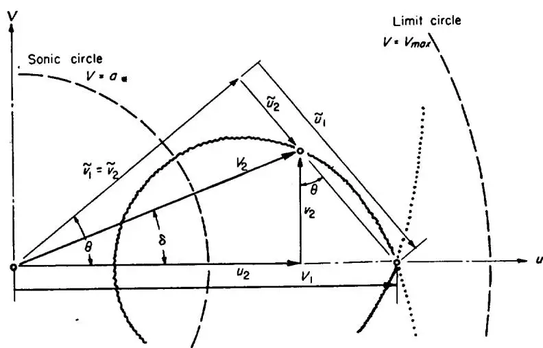
SHOCK POLAR
The velocities associated with an oblique shock wave are conveniently represented in the velocity-vector (hodograph) plane. For a given Mach number ahead of the shock wave, all possible velocity vectors behind the shock lie on a single curve.
Only the closed loop represents real shock waves with non-decreasing entropy, and forms Busemann's shock polar (fig. 3). Its equation is
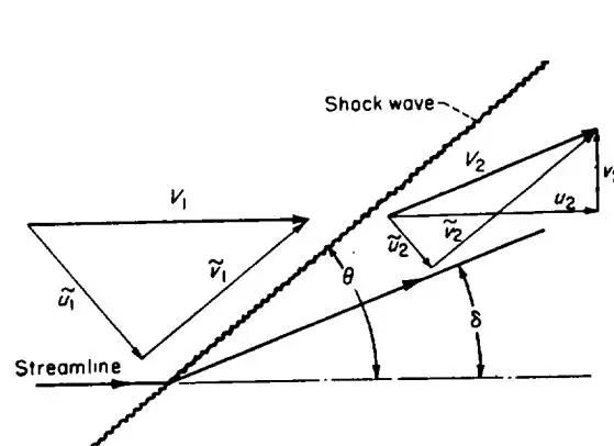
A diagram illustrating the velocity components and angles across a shock wave. On the left, a streamline is shown with a velocity vector v1 and its components v~1 and u~1. On the right, a shock wave is shown with a velocity vector v2 and its components v~2 and u2. The angle between the streamline and the shock wave is θ, and the angle between the streamline and the normal to the shock wave is δ.
Shock wave
v1
v~1
u~1
Streamline
v2
v~2
u2
θ
δ
Scientific illustration: Velocity vectors and angles across a shock wave.
A diagram in the u-v plane showing a velocity vector triangle. The horizontal axis is u and the vertical axis is v. A vector v1 points from the origin to a point on the u-axis. A vector v2 points from that point to a point in the first quadrant. A vector v~1=v~2 points from the origin to the same point in the first quadrant. The angle θ is between the u-axis and the vector v1. The angle δ is between the u-axis and the vector v~1=v~2. The angle θ is also between the vector v2 and the vertical axis. A dashed circle labeled "Sonic circle" V=a is centered at the origin. A solid circle labeled "Limit circle" V=Vmax is centered at a point on the u-axis. A dotted line passes through the point on the u-axis where the limit circle is centered.
Scientific illustration: Velocity vector triangle with sonic and limit circles in u-v plane.
For small deflection angles (hence Mach numbers close to unity), the deflection angle (radians) for sonic flow behind the shock is given approximately in terms of the upstream Mach number by
In unsteady flow all the above relations are valid across a moving oblique shock wave if instantaneous velocities are measured relative to the shock.
SUPERSONIC FLOW PAST WEDGES AND CONES
A shock wave forms ahead of any body in supersonic flight and remains fixed relative to the body if the flight is steady. It stands ahead of blunt shapes, but may be attached to pointed shapes.
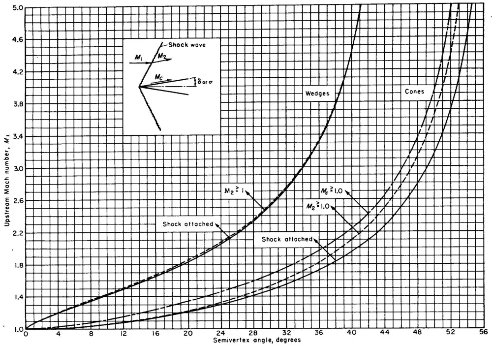
Just at the tip of a pointed airfoil or body of revolution the flow is the same as for the initially tangent wedge or cone. The bow wave is attached at sufficiently high Mach numbers for a wedge of semivertex angle δ less than sin−1(1/γ)=45.6∘ for γ=7/5, and for a circular cone of semivertex angle σ less than 57.5∘ for γ=1.405. Below these limits, the wave is attached above a minimum Mach number whose dependence upon nose angle is shown for wedges and cones in figure 4. (These values can be applied to pointed airfoils and bodies of revolution which are not concave.) Also shown in figure 4 are the slightly higher Mach numbers above which the velocity behind the shock wave is supersonic, and for the cone the still higher Mach number above which the flow is supersonic even at the surface. (For wedges these last two coincide.) For thin wedges, these Mach numbers are given approximately by equations (169) and (170).
FLOW PAST WEDGES
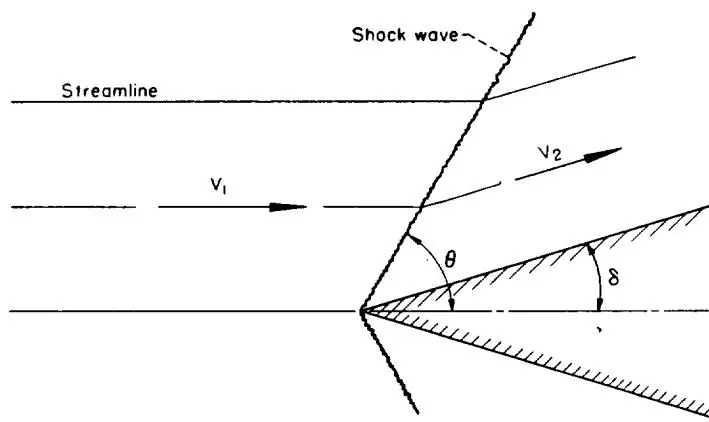
If the bow shock wave is attached to a wedge, it is straight, and the flow behind the shock consists of uniform streams parallel to either face of the wedge. The flow pattern above the upper face (fig. 5) may be regarded as obtained from the straight oblique shock-wave pattern of figure 2 by replacing the streamline behind the shock wave with a solid wall. Flow quantities are determined by the oblique-shock-wave relations, equations (115) to (170). As noted previously, table II can also be applied if M1sinθ is used in place of M1 in the first column.
The flows above and below the wedge are independent, so that inclined wedges can be treated if neither face exceeds the attachment angle shown in figure 4. However, if the angle of attack exceeds the semivertex angle, the flow over the upper (leeward) surface is given by a Prandtl-Meyer expansion (see fig. 4) rather than by the shock relations.
It is clear from the shock polar (fig. 3) that two different shock waves and flow patterns are theoretically possible for a given wedge and Mach number. However, it is believed that only the weaker shock wave (larger u2 and smaller θ) can occur attached to an isolated convex body.
Charts 2, 3, and 4 show the dependence of shock-wave angle, surface pressure coefficient, and downstream Mach number upon wedge angle for various free-stream Mach numbers.
FLOW PAST CONES
If the bow shock wave is attached to an uninclined circular cone, the shock wave too has the form of a circular cone. Flow quantities are constant on all concentric conical surfaces lying between the shock wave and the body, and so depend upon only one space variable. The transition across the shock wave is governed by the oblique-shock relations,
This graph plots the Upstream Mach number, M1, on the y-axis (ranging from 1.0 to 5.0) against the Semivertex angle, degrees, on the x-axis (ranging from 0 to 56). The chart shows several curves representing different shock wave conditions and a wedge.
Key features and labels:
Shock wave diagram: An inset diagram shows a shock wave with upstream Mach number M1, downstream Mach number M2, and critical Mach number Mc. The angle δ or σ is indicated.
Wedges: A solid curve representing the boundary of a wedge.
Cones: Dashed and dash-dotted curves representing cones.
Shock attached: A solid curve labeled "Shock attached" for M2≥1.
Shock detached: A dashed curve labeled "Shock attached" for M2≥1.0.
Critical Mach number: A dash-dotted curve labeled Mc≥1.0.
Semivertex angle, degrees
Wedge (M2≥1)
Cone (M2≥1.0)
Cone (Mc≥1.0)
0
1.0
1.0
1.0
4
~1.15
~1.05
~1.0
8
~1.35
~1.25
~1.05
12
~1.55
~1.45
~1.15
16
~1.75
~1.65
~1.25
20
~1.95
~1.85
~1.35
24
~2.15
~2.05
~1.45
28
~2.35
~2.25
~1.55
32
~2.55
~2.45
~1.65
36
~2.75
~2.65
~1.75
40
~3.0
~2.85
~1.85
44
~3.5
~3.15
~2.0
48
~4.0
~3.5
~2.2
52
~5.0
~4.5
~2.5
Line chart: Upstream Mach number versus semivertex angle for shock waves and wedges.
FIGURE 4.—Upstream Mach numbers for shock attachment and for supersonic flow behind shock wave on wedges and cones, and for supersonic flow at surface of cones.
A diagram showing a flow field with a streamline (horizontal line) and a shock wave (angled line) originating from a wedge. The velocity vector v1 is shown before the shock, and v2 is shown after it. The angle between the streamlines is θ, and the angle between the shock and the horizontal is δ. The wedge is represented by hatched lines.
Shock wave
Streamline
v1
v2
θ
δ
Scientific illustration: Oblique shock wave and streamlines around a wedge.
FIGURE 5.—Flow past a wedge.
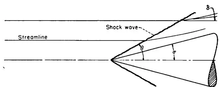
and is followed by a continuous isentropic compression to surface conditions, as indicated in figure 6. The flow quantities have been extensively tabulated in reference 6 for γ=1.405 and for γ=4/3. As in the case of wedges, two solutions exist for each cone and Mach number, but it is believed that only the weaker shock wave can occur on an isolated convex body. Charts 5, 6, and 7 show the dependence of shock-wave angle, surface-pressure coefficient, and
A diagram showing streamlines (horizontal lines) and a shock wave (a thick, curved line) emanating from a point on the right. The angles δ, θ, and σ are marked. A shaded region is shown at the bottom right.
Streamline
Shock wave
δ
θ
σ
Scientific illustration: Shock wave and streamlines around a body with angles delta, theta, and sigma.
FIGURE 6.—Flow past a cone.
surface Mach number on cone semivertex angle for various free-stream Mach numbers.
The effects of slightly inclining a cone have been considered by Stone (ref. 13) and numerical results are tabulated in reference 14. Chart 8 shows the variation with Mach number of the initial slope of the normal-force curve for various cone angles. Stone has also sought an approximation for larger inclinations by retaining squares as well as first powers of angle of attack (ref. 15), and numerical results have been tabulated (ref. 16); however, these results are not free of error (see refs. 17 and 18).
PRANDTL-MEYER EXPANSION
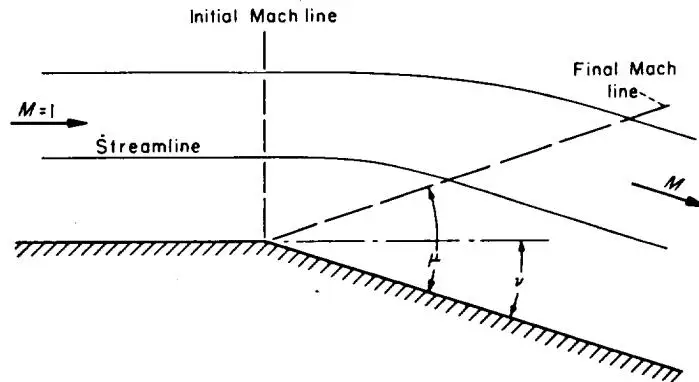
A uniform two-dimensional supersonic stream flowing over a convex bend expands isentropically. Convenient relations are found by considering the special case of a stream at Mach number unity flowing around a sharp corner (fig. 7).
Initial Mach line
Final Mach line
M=1
Streamline
M
μ
ν
A diagram showing a streamline and two Mach lines (initial and final) over a wedge surface. The initial Mach line is vertical. The final Mach line is dashed. The angle between the streamline and the final Mach line is labeled μ. The angle between the final Mach line and the surface is labeled ν. A horizontal arrow labeled M=1 points to the left, and a horizontal arrow labeled M points to the right.
Scientific illustration: Mach lines and streamline over a wedge surface.
FIGURE 7.—Prandtl-Meyer expansion around a corner.
For a perfect gas, the Prandtl-Meyer angle ν through which the stream turns in expanding from M=1 to a supersonic Mach number M is
which falls to zero as ν→νmax. Numerical values of ν, μ, and p/pi are given in table II as functions of M.
These relations and the values in table II apply to a uniform stream flowing past any convex surface in the ab-
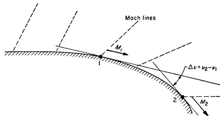
sence of external disturbances. (They also give a very good approximation at all Mach numbers when, as on an airfoil, external disturbances arise only from interaction with a shock wave, and are disregarded.) If flow quantities are known at one point, the values at any second point can be read from table II by identifying the change in flow angle between the two points with Δν=ν2−ν1, as indicated in figure 8.
Mach lines
M1
1
Δv=v2−v1
2
M2
A diagram showing a curved surface with two points, 1 and 2. Mach lines are represented by dashed lines. At point 1, a velocity vector M1 is shown. At point 2, a velocity vector M2 is shown. The change in velocity is indicated as Δv=v2−v1.
Scientific illustration: Mach lines and velocity change across a curved surface.
FIGURE 8.—Prandtl-Meyer expansion over a convex surface.
For expansions through small angles Δν, the ratio of final to initial static pressures is given by the following series (Δν in radians):
Up to and including the term in (Δν)2 this series is identical with that for compression through an oblique shock wave (eq. (151) with δ=−Δν).
IMPERFECT-GAS EFFECTS
Methods for calculating the flow of a calorically imperfect, thermally imperfect gas and a calorically imperfect, thermally perfect gas at temperatures up to 5000∘ R are described in this section. The equations presented are in substantially the same form as those given in references 7 and 8. Effects of gaseous imperfections, such as molecular dissociation, which become important at temperatures greater than about 5000∘ R are not considered.
Atmospheric and wind-tunnel air flows are of primary concern here. In such flows air generally exhibits only caloric imperfections to any appreciable degree. Consequently, numerical results are presented only for the flow of a calorically imperfect, thermally perfect diatomic gas.
THERMODYNAMICS
EQUATIONS OF STATE
The thermal equation of state used here for a calorically and thermally imperfect gas is the Berthelot equation
(eq. (5)). The thermal equation of state used for a calorically imperfect, thermally perfect gas is equation (2). The caloric equation of state used for a calorically and thermally imperfect gas is equation (8a). The caloric equation of state used for a calorically imperfect, thermally perfect gas is equation (8b).
SPECIFIC HEATS
The assumption of a simple harmonic vibrator is used to account for the contribution of the vibrational heat capacity to the specific heats. The equations for the specific heats at constant volume and constant pressure, respectively, are (see ref. 7)
The following values of γ are for temperatures from 400° R to 5000° R, with Θ=5500∘ R (see ref. 7). For engineering purposes, these are a satisfactory approximation for air.
VARIATION OF RATIO OF SPECIFIC HEATS WITH TEMPERATURE
T,∘R
γ
T,∘R
γ
T,∘R
γ
500
1.400
1300
1.361
2200
1.322
600
1.399
1400
1.355
2400
1.317
700
1.396
1500
1.349
2600
1.313
800
1.392
1600
1.344
2900
1.309
900
1.387
1700
1.339
3000
1.306
1000
1.381
1800
1.335
3500
1.301
1100
1.375
1900
1.331
4000
1.298
1200
1.368
2000
1.328
4600
1.296
5000
1.294
CONTINUOUS ONE-DIMENSIONAL FLOW
BASIC EQUATIONS AND DEFINITIONS
Basic equations pertinent to this section are equations (26), (27), (28), (29), (30), and (31). The equations for the speed of sound are (see ref. 7)
The variations of (a∗V)perf(a∗V)therm perf and (TtT)perf(TtT)therm perf with Mach number for several values of total temperature Tt are given in charts 9 and 10.
PRESSURE AND DENSITY RELATIONS
For isentropic flow, the relations between density and temperature are (see ref. 7)
The variation of (ρtρ)perf(ρtρ)therm perf with Mach number for several total temperatures is presented in chart 11.
For the isentropic flow of a thermally imperfect, calorically imperfect gas, the relation between pressure, density, and temperature can be obtained by a trial-and-error procedure using equations (5) and (187).5 For the isentropic flow of a thermally perfect gas, the relation between pressure and temperature is
The relation between dynamic and static pressure for a thermally imperfect gas can be obtained by a trial-and-error procedure using equations (5), (31a), (183), and (187). The relation between dynamic and static pressure for a thermally perfect gas can be obtained with equations (31b) and (186), and is
The variations of (ptp)perf(ptp)therm perf and (ptq)perf(ptq)therm perf with Mach
number for several total temperatures are given in charts 12 and 13.
STREAM-TUBE-AREA RELATIONS
The stream-tube-area relation is given by equation (79), or, in more convenient form,
A∗A=ρaMρ∗a∗(191)
This ratio can be evaluated for a thermally imperfect gas with the aid of equations (187), (181), (5), and (185), and for a thermally perfect gas with the aid of equations (188),
(182), and (186). The variation of (A∗A)perf(A∗A)therm perf with Mach
number for several values of total temperature is presented in chart 14.
5 In this, as in many of the cases to be presented, no direct solution for flow properties is possible if the gas exhibits both thermal and caloric imperfections. Approximate solutions of this type can be obtained, however, if the degree of imperfection is small (see ref. 7).
NORMAL SHOCK WAVES
The requirements for conservation of mass, momentum, and energy across a normal shock wave are given by equations (84), (85), and (86a). The energy relation can be written
No explicit equation has been found to relate the temperature downstream of a normal shock wave in thermally imperfect air to the upstream conditions. A trial-and-error procedure, starting with assumed values of ρ2 and T2 and involving equations (5), (84), (85), and (192), can be used to determine the downstream temperature.
For the flow of a thermally perfect gas, the simultaneous solution of equations (84), (85), (193), and (2) yields the following relation from which the temperature behind the shock wave can be found:
Since the total temperature Tt remains constant across a shock wave, other flow parameters behind the shock wave can be found with the aid of previously presented one-dimensional flow relations. The variations of
(T1T2)pert(T1T2)therm perf,(ρ1ρ2)pert(ρ1ρ2)therm perf,(pt2p1)pert(pt2p1)therm perf,(p1p2)pert(p1p2)therm perf,M2pertM2therm perf, and (pt1pt2)pert(pt1pt2)therm perf
with upstream Mach number for several total temperatures are presented in charts 15 through 20, respectively.
OBLIQUE SHOCK WAVES
For a thermally imperfect gas, no simple equations can be found to relate the values of the flow parameters across oblique shock waves. In general, trial-and-error procedure, starting with assumed values of ρ2 and T2, and involving the relations for the conservation of mass, momentum, and energy, must be used. (See eqs. (115), (116), (117), and (118a) as well as equations (5) and (183).) For a thermally perfect gas, the Mach number downstream of an oblique shock wave can be found with the aid of the energy equation (see eqs. (118a) and (186)), thus
The density ratio can be determined from the equation of state (eq. (2)) with the aid of the pressure and temperature ratios. The shock-wave and deflection angles are given by (see ref. 8)
The variation of θ with δ for various values of M1 and T1 is presented in chart 21. In addition, the variations of
(M2)pert(M2)therm perf and (q1p2−p1)pert(q1p2−p1)therm perf with δ for various M1 and T1
are presented in charts 22 and 23.
Values of the ratios
p1p2,ρ1ρ2,T1T2,pt1pt2
for the flow of a thermally perfect gas across an oblique shock wave can be determined from the normal-shock relations,
provided that M1sinθ is used instead of M1 and that the static temperature T1 just upstream of the shock wave is the same for the oblique shock wave as for the normal shock wave.
PRANDTL-MEYER EXPANSION
The Prandtl-Meyer angle for the flow of an imperfect gas can be found by graphically integrating the equation (see ref. 8)
ν=−∫p∗pρV2tanμdp[isen](199)
The relations between p, ρ, V, and μ can be found with the
aid of equations (5), (187), (183), and (185). For a thermally perfect gas this equation becomes (see, again, ref. 8)
ν=−∫p∗p2γpsin2μdp[isen, therm perf](200)
The relations between γ, p, and μ can be found with the aid of equations (180), (189), and (186) using the temperature as a parameter. The graphical integration of equation (200) has been carried out, and the variations of νtherm perf and νperfνtherm perf with Mach number for various values of total temperature are presented in chart 24.
APPENDIX A
VISCOSITY AND THERMODYNAMIC CONSTANTS FOR AIR
VISCOSITY
The viscosity of air is nearly independent of pressure; the variation with absolute temperature, between temperatures of about 300° R and 900° R, may be approximated by the formula
μrμ=(TrT)0.76(A1)
For a wider range of temperatures, between about 180° R and 3400° R, Sutherland's formula (see ref. 19) is more accurate:
μrμ=T+198.6Tr+198.6(TrT)3/2(A2)
The viscosity of air, as determined from this relation, may be expressed as
μ=2.270T+198.6T3/2×10−8ft2lb sec(A3)
This latter equation has been employed in the calculations of Reynolds number (chart 25).
THERMODYNAMIC CONSTANTS
The value of γ employed for air, when treated as a completely perfect gas, is 7/5. This simple value, which has been employed in table I, table II, charts 1 to 4, and chart 25, is a good approximation to the more precise values obtained from spectroscopic measurements (see ref. 20). Values of cp, cv, and R for air, consistent with the approximation γ=7/5, are
 Fiber
 Connect
 Omnipub
 What the PDF's own text says
 What the PDF's own text says
 1960 · English · first 20 of 36 pages
 1953 · English · first 20 of 70 pages
 2016 · English · 16 pages
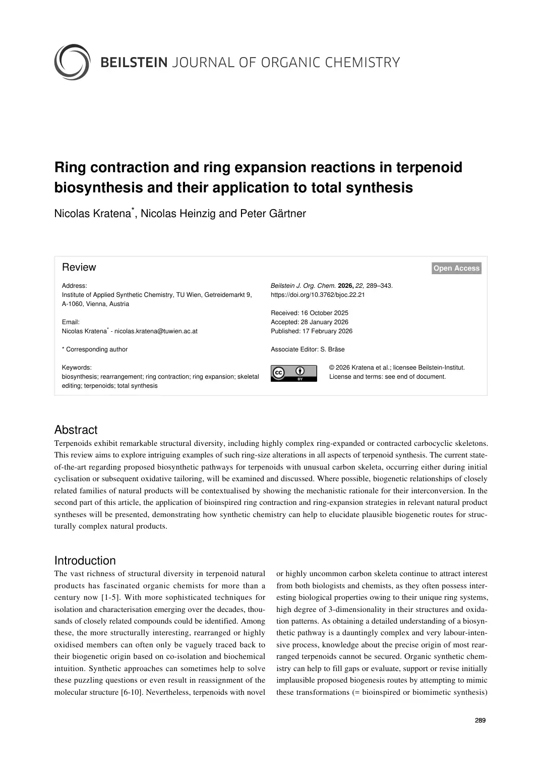 2026 · English · first 20 of 55 pages
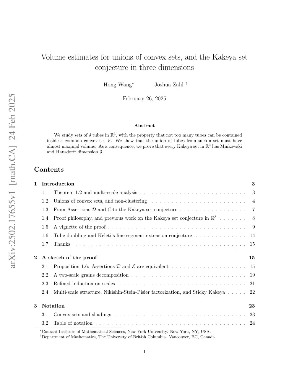 2025 · English · first 20 of 127 pages
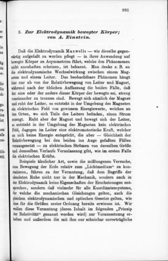 1905 · German · first 20 of 31 pages