Your catalog was built for people to find. Now AI has to understand it.
Most publishers hold thousands, often millions, of PDFs, laid down in layers over thirty years. Each layer solved the problem of its day.
1990s
You went digital
The paper archive was scanned into PDFs, one picture per page. The pages survived. What was on them, to software, did not.
Old or new, your PDFs weren't made for AI.
A scan from 1960 and a PDF from last month fail in different ways, but both fail. Getting your corpus ready means more than better OCR: every page has to be rebuilt as a document an AI can navigate, quote, and credit. That is what Cashmere does, for every PDF you hold.
The problem
Not all PDFs are created equal
Whether software can read a PDF depends on how it was made, and the oldest files, often the most valuable in a catalog, are the hardest of all. Here is one equation from each kind, three ways.
1
Hard
Born digital
LIGO 2016 · Kakeya 2025 · Beilstein 2026
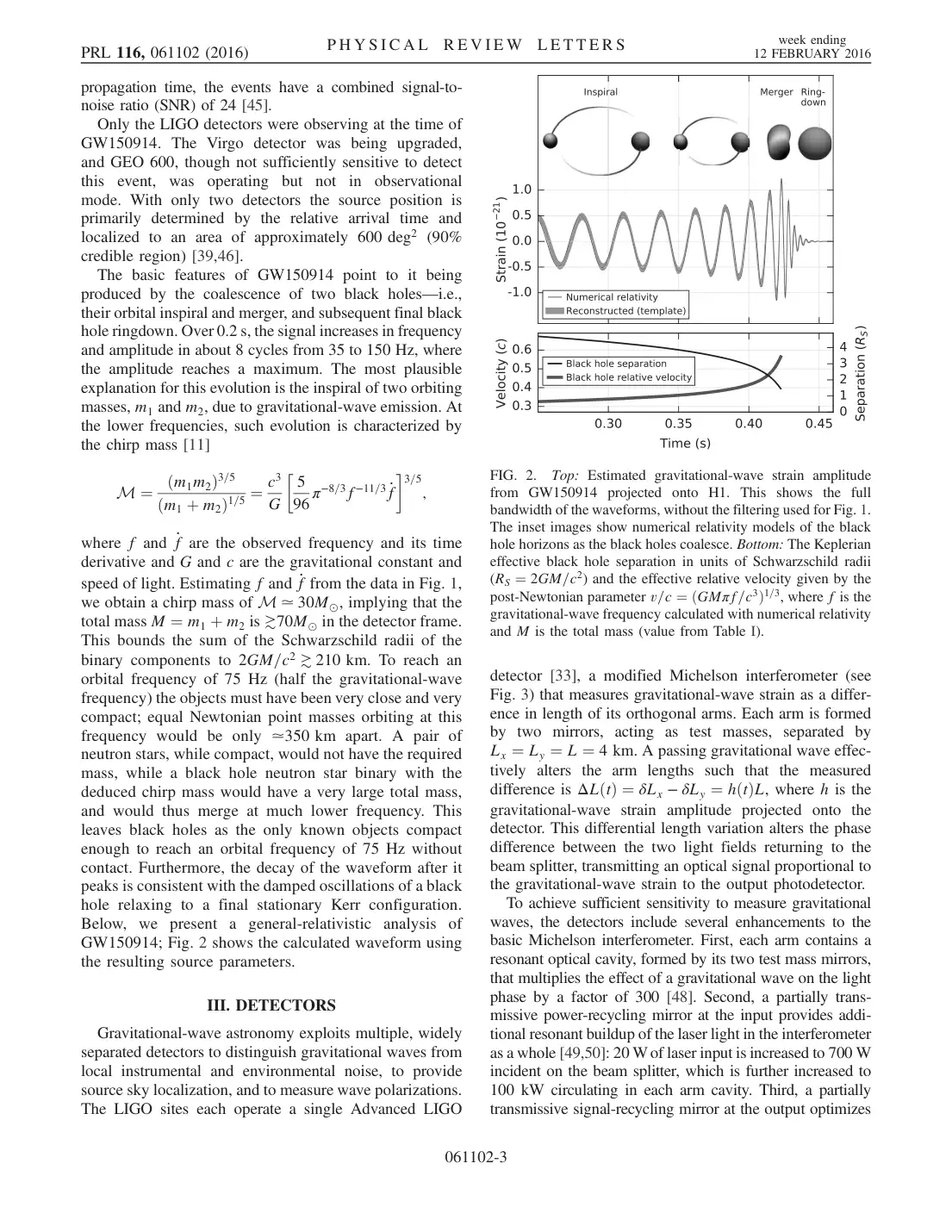
The text is real, but it is stored as letters placed on a page, in the font’s own private encoding. Fractions fall apart, = becomes ¼, and a two-column page reads straight across both columns.
The page
What the PDF's own text says
M ¼ ðm1m2Þ3=5 ðm1 þ m2Þ1=5 ¼ c3 G 5 96 π−8=3f−11=3 _f 3=5 ;
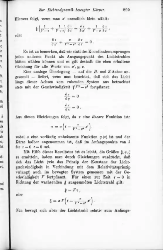
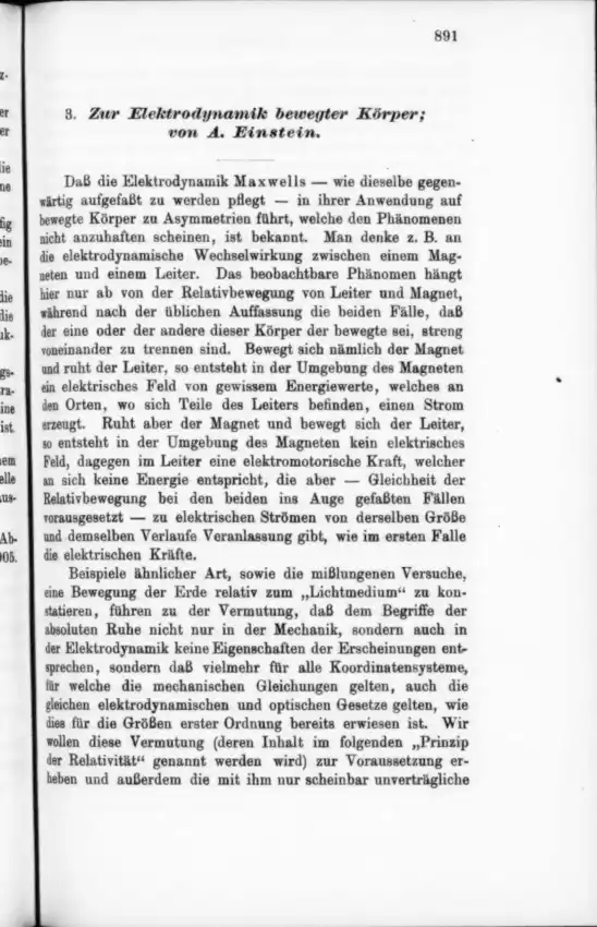
A photograph of a printed page. The only text is an OCR layer added later, which reads ordinary words and gives up on everything else: equations, tables, and symbols.
The page
What the PDF's own text says
=
Ot
Or
9:
oder
let.
OCR layer: fragments
What the omnipub says
21(V−v1+V+v1)∂t∂τ=∂x′∂τ+V−v1∂t∂τ,
∂x′∂τ+V2−v2v∂t∂τ=0.
Einstein, 1905, page 9
3
Hardest
Typewritten originals
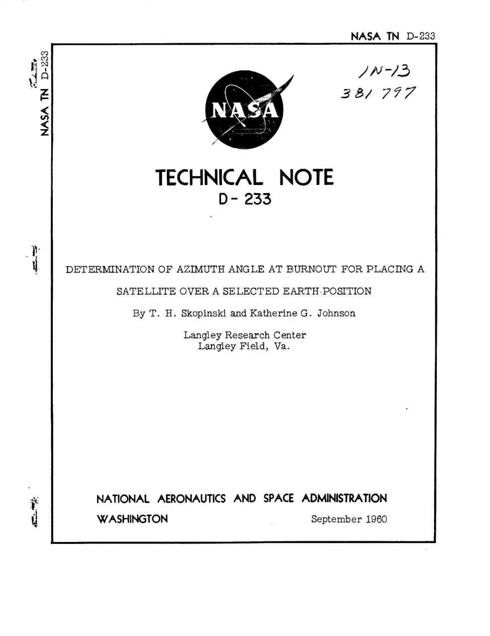
NASA TN D-233, Katherine Johnson, 1960
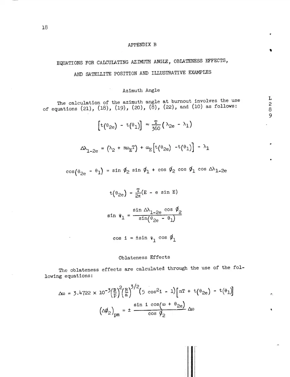
Typed, copied, and scanned from the copy. Uneven strikes, stamps, and margin notes, and Greek letters the OCR never learned: every λ, ω, and θ below is lost or misread.
The page
What the PDF's own text says
2_i_2e = (h2 + r_oET) + _E[t(e2e) -t(el)] - h I
OCR layer: symbols lost
What the omnipub says
Δλ1−2e=(λ2+nωET)+ωE[t(θ2e)−t(θ1)]−λ1
NASA TN D-233, 1960, page 20
Why it matters
AI can only use what it can read.
A paper that fails ingestion is invisible: it can’t be searched, retrieved, cited, or licensed.
Wrong is worse than missing.
A misread number in a table or a garbled equation doesn’t look broken to an AI. It gets quoted, confidently.
The back catalog is the hard part.
Decades of scanned journals, reports, and books hold a publisher’s most distinctive content, and they are the nastiest PDFs of all.
How it works
From a page of ink to a document AI can use
One page of Katherine Johnson’s 1960 NASA paper, all the way through Cashmere. Every picture below is the real page and the real output.
STEP 01
Start with a PDF
A PDF records where ink goes on a page. To software, this page is a picture: the equations aren't text at all, and its OCR layer reads them as noise.
STEP 02
Read the page like a person
The Pro parser finds the structure a reader sees: which marks are a heading, a paragraph, an equation, a table, or a figure, and the order they're read in.
heading26
paragraph235
equation84
table11
figure13
list item24
787 blocks in the whole paper
STEP 03
Make every piece a block
Each piece becomes an omnipub block with a type and a stable address, so it can be searched, quoted, cited, and licensed on its own. Equations become real math.
Contents
SUMMARY3
INTRODUCTION4
SYMBOLS102
SATELLITE POSITION RELATIONSHIPS5
EXPRESSION FOR PLACING A SATELLITE OVER A SELECTEDPOSITION27
APPENDIX B1
EQUATIONS FOR CALCULATING AZIMUTH ANGLE, OBLATENESS EFFECTS,AND SATELLITE POSITION AND ILLUSTRATIVE EXAMPLES1
The blocks are put back together as the paper itself: sections inside sections, in reading order, each with its own address. The result is one document an AI can navigate and measure, from its table of contents down to a single equation.
Every block remembers where it sat on the original page. An answer can cite the exact equation it used, and anyone can check it against the source.
Pick a paper below to see every page and every block side by side.
Why Cashmere
Parsed isn’t the same as AI-ready
Plenty of tools can pull text out of a PDF. An AI needs more: what each piece is, where it belongs, where it came from, and what it may be used for. That is the work Cashmere does, on the files other pipelines give up on.
Right on the hard pages
Layout, text, math, and tables are read from the page image itself, not from the broken text layer, so a 1905 scan comes out as clean as a 2025 preprint.
Structured like the work
Headings, sections, and reading order are kept, and every block gets a stable address. An AI can find the right passage instead of guessing from a wall of text.
Traceable to the source
Every block keeps its place on the original page. An answer can cite the exact paragraph or equation it used, and anyone can check it.
Licensed and measured
Rights travel with the content, and use is counted block by block, so you know what AI systems read and you get paid for it.
6 papers, 335 pages, from a 1905 scan to a 2025 preprint, converted by one pipeline with no hand corrections. Bring us your hardest PDFs.
Converted by Cashmere’s Pro parser, November 2026, and shown without hand corrections.
Thousands of PDFs or millions, ready for AI.
Cashmere converts your entire corpus quickly and accurately, from decades-old scans to last month’s releases, so AI can read it, cite it, and credit you.
Opening the paper. Everything you’re about to see is Cashmere’s first pass at this PDF. Nobody touched it up, so this is exactly what the pipeline does.
Volume estimates for unions of convex sets, and the Kakeya set conjecture in three dimensions
Scanned PDF
page 1 / 20
OmnipubClick any block to see its data
Volume estimates for unions of convex sets, and the Kakeya set conjecture in three dimensions
Hong Wang* Joshua Zahl†
February 26, 2025
Abstract
We study sets of δ tubes in R3, with the property that not too many tubes can be contained inside a common convex set V. We show that the union of tubes from such a set must have almost maximal volume. As a consequence, we prove that every Kakeya set in R3 has Minkowski and Hausdorff dimension 3.
Contents
1
Introduction
3
1.1
Theorem 1.2 and multi-scale analysis . . . . .
3
1.2
Unions of convex sets, and non-clustering . . . . .
4
1.3
From Assertions D and E to the Kakeya set conjecture . . . . .
7
1.4
Proof philosophy, and previous work on the Kakeya set conjecture in R3 . . . . .
8
1.5
A vignette of the proof . . . . .
9
1.6
Tube doubling and Keleti’s line segment extension conjecture . . . . .
14
1.7
Thanks . . . . .
15
2
A sketch of the proof
15
2.1
Proposition 1.6: Assertions D and E are equivalent . . . . .
Move #3: Replacing grains with wider grains with small CKT−CWloc . . . . .
85
9
A refined induction-on-scales argument
100
10
Sticky Kakeya for tubes satisfying the Katz-Tao Convex Wolff Axioms at every Scale
103
10.1
Nikishin-Stein-Pisier Factorization and the Convex Wolff Axioms . . . . .
105
11
Multi-scale analysis and the proof of Proposition 1.7
110
12
Tube Doubling
114
A A grains decomposition for tubes in R3
115
B Wolff’s hairbrush argument and the proof of Proposition 1.8
125
1 Introduction
A Kakeya set is a compact subset of Rn that contains a unit line segment pointing in every direction. The Kakeya set conjecture asserts that every Kakeya set in Rn has Minkowski and Hausdorff dimension n. This conjecture was proved by Davies [5] when n=2, and is open in three and higher dimensions. See [17, 28] for an introduction to the Kakeya conjecture and a survey of historical progress on the problem. See [15, 16, 18, 20, 21, 27, 31] for current progress towards the conjecture in three and higher dimensions.
The purpose of this paper is to obtain lower bounds on the volume of unions of δ-tubes (i.e. the δ neighbourhoods of unit line segments) in R3 that satisfy certain non-clustering conditions. As a consequence, we resolve the Kakeya set conjecture in three dimensions.
Theorem 1.1.Every Kakeya set in R3 has Minkowski and Hausdorff dimension 3.
Theorem 1.1 is a corollary of the following slightly more technical result.
Theorem 1.2.For all ε>0, there exists K>1 so that the following holds for all δ>0 sufficiently small. Let T be a set of δ-tubes contained in the unit ball in R3, and suppose that every rectangular prism of dimensions a×b×2 contains at most 100abδ−2 tubes from T (this is true, for example, if the tubes in T point in δ-separated directions). For each T∈T, let Y(T)⊂T be a measurable set with ∣Y(T)∣≥λ∣T∣. Then
T∈T⋃Y(T)≥δελKT∈T∑∣T∣.(1.1)
The Kakeya maximal function conjecture asserts that for each ε>0, Inequality (1.1) is true for K=3. The Kakeya maximal function conjecture in R2 was proved by Cordoba [6]. While we do not resolve the Kakeya maximal function conjecture in R3, the weaker statement given in Theorem 1.2 is nonetheless sufficient to obtain Theorem 1.1.
The hypothesis that each a×b×2 rectangular prism contains at most 100abδ−2 tubes from T is a type of non-clustering condition. A close variant of this hypothesis was first introduced by Wolff in [27], and sets of tubes that satisfy this hypothesis are said to satisfy the Wolff axioms.
1.1 Theorem 1.2 and multi-scale analysis
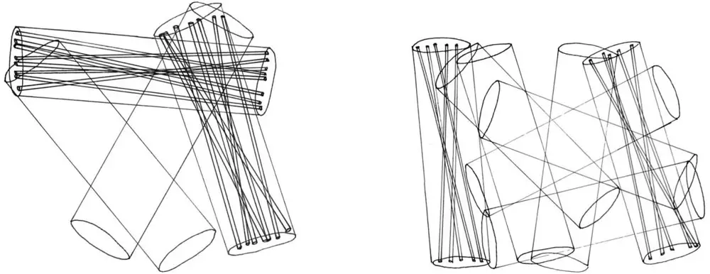
In [25, 26], the authors showed that Theorem 1.2 is true when the set T has a property called stickiness (see Figure 1 (left)). Roughly speaking, T is sticky if it satisfies the non-clustering condition from Theorem 1.2; has cardinality roughly δ−2; and for every intermediate scale δ≤ρ≤1, the tubes in T can be covered by a set of ρ tubes that satisfy the non-clustering condition from Theorem 1.2 with ρ in place of δ.
Unfortunately, not every set of tubes is sticky — see Figure 1 (right) for an example. The arrangement illustrated in Figure 1 (right) is challenging to analyze, because the ρ tubes intersect with large multiplicity (i.e. many ρ tubes pass through a typical point), but the arrangement of
Two side-by-side diagrams show a 3D geometric configuration of four intersecting cylinders. In the left diagram, blue lines connect points on the cylinders in a specific pattern. In the right diagram, the same cylinders are shown with blue lines connecting points in a different pattern. The cylinders are drawn with black outlines and the lines are drawn in blue.
The image consists of two side-by-side diagrams. Each diagram shows four intersecting cylinders. In the left diagram, blue lines connect points on the cylinders in a specific pattern. In the right diagram, the same cylinders are shown with blue lines connecting points in a different pattern. The cylinders are drawn with black outlines and the lines are drawn in blue.
Scientific illustration: Geometric illustration of intersecting cylinders with blue lines connecting points.
Figure 1: Left: The tubes at scale ρ (black) satisfy the non-concentration hypothesis of Theorem 1.2, as do the (rescaled) δ tubes (blue) inside each ρ tube. Multi-scale analysis is straightforward in this setting. This is sometimes called the “sticky” case. For clarity, not all δ tubes have been drawn.
Right: The tubes at scale ρ do not satisfy the non-concentration hypothesis of Theorem 1.2. The tubes at scale ρ intersect with high multiplicity, while the δ tubes inside each ρ tube are sparse.
δ tubes inside each ρ tube is sparse (i.e. the union of δ tubes inside each ρ tube only fill out a small fraction of that ρ tube). To help us analyze this type of arrangement, in Section 1.2 we will introduce two variants of the non-clustering hypothesis from Theorem 1.2, and two variants of the volume estimate (1.1).
1.2 Unions of convex sets, and non-clustering
In what follows, we say a pair of sets U,V⊂Rn are essentially distinct if ∣U∩V∣≤21max(∣U∣,∣V∣). T will denote a set of essentially distinct δ-tubes contained in the unit ball in R3, and ∣T∣ will denote the volume of a δ-tube, i.e. ∣T∣ has size about δ2.
Definition 1.3. Let T be a set of δ-tubes in R3.
(A) We define CKT−CW(T) to be the infimum of all C>0 such that
#{T∈T:T⊂W}≤C∣W∣∣T∣−1for all convex sets W⊂R3.
We say that T obeys the Katz-Tao Convex Wolff Axioms with error CKT−CW(T).
(B) We define CF−SW(T) to be the infimum of all C>0 such that
#{T∈T:T⊂W}≤C∣W∣(#T)for all slabs W⊂R3,
where a “slab” is the intersection of the unit ball with the thickened neighbourhood of a (hyper) plane. We say that T obeys the Frostman Slab Wolff Axioms with error CF−SW(T).
Remark 1.4.
(A) A note on etymology. The terms “Katz-Tao” and “Frostman” refer to different types of non-concentration conditions; they are the analogues of the well-studied non-concentration conditions
∣E∩B∣≤(r/δ)2 and ∣E∩B∣≤r2∣E∣, where E⊂Rn is a δ-separated set and B is a ball of radius r. An arrangement of tubes arising from a Kakeya set, i.e. a set of δ-tubes with one tube pointing in each δ-separated direction, obeys both the Katz-Tao Convex Wolff Axiom and Frostman Slab Wolff Axiom with error ≲1. The terms “convex” and “slab” refer to the class of sets for which the non-clustering condition is imposed. The term “Wolff axioms” suggests that the above definition is an analogue of the Wolff axioms from [27].
(B) The above definitions are two special cases of a non-clustering condition (Definition 1.3') that will be defined in Section 4.2. In Definition 1.3', both tubes and convex sets (resp. slabs) are replaced by more general objects.
(C) If T is non empty, then by taking W to be a δ×1×1-slab containing a tube of T, we can see CF−SW(T)≤C implies #T≥C−1δ−1.
Next, we introduce two Kakeya-type volume estimates for unions of tubes in R3. These are analogues of Inequality (1.1) that are carefully formulated to be amenable to induction on scale. In what follows, we use the notation (T,Y)δ to denote a collection T of essentially distinct δ-tubes in R3, and a shading of these tubes, i.e. for each T∈T, Y(T) is a subset of T. For λ>0, we say (T,Y)δ is λdense if ∑T∈T∣Y(T)∣≥λ∑T∈T∣T∣.
Definition 1.5. Let σ,ω≥0.
• We say that Assertion D(σ,ω) is true if the following holds: For all ε>0, there exists κ,η>0 such that the following holds for all δ>0. Let (T,Y)δ be δη dense and obey the Katz-Tao Convex Wolff Axioms and Frostman Slab Wolff Axioms, both with error at most δ−η. Then
T∈T⋃Y(T)≥κδω+ε(#T)∣T∣((#T)∣T∣1/2)−σ.(1.2)
• We say that Assertion E(σ,ω) is true if the following holds: For all ε>0, there exists κ,η>0 such that the following holds for all δ>0. Let (T,Y)δ be δη dense. Then
Let us examine the numerology in the estimates (1.2) and (1.3). First, in the special case σ=ω, Assertion D(σ,σ) yields the estimate
T∈T⋃Y(T)≥κδε(#T)−σT∈T∑∣T∣,
i.e. it says that there are ≲δ−ε(#T)σ tubes passing through a typical point of the union ⋃Y(T) (for general σ and ω, this quantity is about δσ−ω−ε(#T)σ). For σ>0 small, this means that the tubes in the union ⋃Y(T) are almost disjoint. In the arguments that follow, it will be helpful to consider situations where σ and ω are not necessarily equal.
The shape of the estimate (1.2) is motivated in part by the following consideration. To begin our induction on scale argument, we would like to prove that E(σ,0) holds for some σ∈(0,2/3]. When σ=1/2 and ω=0, Inequality (1.2) becomes the estimate
T∈T⋃Y(T)≥κδ1/2+ε(δ2#T)1/2.
This is essentially Wolff's hairbrush bound from [27] (here we make use of the fact that T obeys the Frostman Slab Wolff Axioms with small error; see Appendix B for details).
Assertion D(σ,ω) is a special case of Assertion E(σ,ω). We will explain the shape of the final bracketed term of Inequality (1.3). To understand the term ℓ, it is helpful to consider the following scenario. Suppose we know that Assertion D(σ,ω) is true. Let δ<ρ<1, and let T be a set of δ tubes of cardinality (ρ/δ)2 that are contained inside a common ρ tube, which we will denote by Tρ. Suppose that the tubes in T obey the Katz-Tao Convex Wolff Axioms with error roughly 1. This implies that CF−SW(T)∼ρ−1.
For T∈T (and hence T⊂Tρ), we will write TTρ to denote the image of T under the affine transformation that anisotropically dilates Tρ by a factor of ρ−1 in its two “short” directions, and translates the image to the unit ball. After this rescaling and translation, the tubes in T become δ/ρ tubes that satisfy the Katz-Tao Convex Wolff Axioms and Frostman Slab Wolff Axioms, both with error roughly 1. Applying Assertion D(σ,ω) to this rescaled collection of tubes, we obtain the volume bound
T∈T⋃TTρ≥κ(δ/ρ)ε(#T)∣TTρ∣((#T)∣Tρ∣1/2)−σ.
Undoing the anisotropic rescaling and translation (which distorted volumes by a factor of ρ2) and noting that ∣TTρ∣∼ρ2∣T∣, we can rewrite this as
As a second justification for the term ℓ, note that for every set T of δ tubes, we must always have CF−SW(T)(#T)∣T∣1/2≥1. This is because we can always select a slab W of thickness ∣T∣1/2 that contains at least one tube from T. This observation also explains the choice to write ∣T∣1/2 rather than δ; any convex set S⊂R3 of diameter 1 can be contained in a slab of thickness ∣S∣1/2. Later in the proof we will consider generalizations of Assertion E(σ,ω) in which tubes are replaced by more general families of convex sets.
To understand the terms m−1 and m−3/2 in Inequality (1.3), it is helpful to consider the following scenario. Suppose we know that Assertion D(σ,ω) is true. Let T be a set of δ tubes that obey the Frostman Slab Wolff Axioms with error roughly 1, and the Katz-Tao Convex Wolff Axioms with error m≫1. Let ρ=m1/2δ, and suppose that there exists a set Tρ of ρ tubes, each of which contains m∣Tρ∣∣T∣−1=m2 tubes from T. Observe that this is the maximum number of essentially distinct δ tubes that can fit inside a ρ tube. In particular, the union of the δ tubes inside each ρ tube fill out essentially all of the ρ tube. We have #Tρ=m−2(#T)=m−1(∣T∣/∣Tρ∣)(#T), i.e. (#Tρ)∣Tρ∣=m−1(#T)∣T∣. It is straightforward to compute that CKT−CW(Tρ)≲1. Applying Assertion D(σ,ω) and using the fact that the union of δ tubes inside each ρ tube fill out most of
1.3 From Assertions D and E to the Kakeya set conjecture
Clearly E(σ,ω)⟹D(σ,ω). In Section 6, we will show that the reverse implication also holds:
Proposition 1.6.Let 0≤σ≤2/3, ω≥0. Then E(σ,ω)⟺D(σ,ω).
As mentioned above, our proof uses induction on scale. In brief, if E(σ,ω) is true, then we will use this fact at many locations and scales to prove that D(σ,ω′) is true for some ω′<ω (observe that smaller values of ω are better). The precise statement is as follows.
Proposition 1.7.There exists a function g:[0,2/3]×(0,1]→(0,1] so that the following is true. Let 0≤σ≤2/3, ω>0. Then E(σ,ω)⟹D(σ,ω−g(σ,ω)).
Propositions 1.6 and 1.7 lead to a self-improving property for E(σ,ω) (or equivalently, for D(σ,ω)). Since the collections of tubes in the definitions of E and D are essentially distinct and are contained in the unit ball, we always have #T≲δ−4, and thus we can “trade” an improvement in ω for an improvement in σ. In particular, Proposition 1.7 tells us that E(σ,ω)⟹D(σ−g(σ,ω)/4,ω).
By applying Propositions 1.6 and 1.7, we can upgrade an initial estimate D(σ,ω) to the improved estimate D(σ−g(σ,ω)/4,ω). We can then iterate this process. In order to begin the iteration, we must prove that D(σ,ω) is true for some ω>0 and 0≤σ≤2/3. In [27], Wolff proved that every Kakeya set in Rn has Hausdorff dimension at least 2n+2. In Appendix B, we will use a similar argument to show that D(1/2,0) is true:
Proposition 1.8.D(1/2,0) is true.
Beginning with Proposition 1.8 and then iterating Propositions 1.6 and 1.7, we conclude the following.
Theorem 1.9.The statements D(0,0) and E(0,0) are true.
Proof. Fix ω>0. By Proposition 1.8, we have that D(1/2,0) and hence D(1/2,ω) is true. If D(σ,ω) is true for some σ∈[0,2/3], then so is D(σ′,ω) for all σ′∈[σ,2/3]. Using Propositions 1.6 and 1.7, we conclude that the set {σ∈[0,2/3]:D(σ,ω) is true} is relatively open in the metric space [0,2/3]. On the other hand, it is straightforward to verify from Definition 1.5 that this set is also relatively closed in [0,2/3]. We conclude that D(σ,ω) is true for all σ∈[0,2/3], so in particular D(0,ω) is true.
A similar argument shows that D(0,0) is true; we have shown that D(0,ω) is true for every ω>0. On the other hand, the set {ω≥0:D(0,ω) is true} is relatively closed in the metric space [0,∞). We conclude that D(0,0) is true. By Proposition 1.6 we have that E(0,0) is true. □
The conclusion of Theorem 1.9 can be rephrased as follows
Corollary 1.10.For all ε>0, there exists K so that the following holds for all δ>0 sufficiently small. Let (T,Y)δ be λ-dense. Then
Theorem 1.2 is now a special case of Corollary 1.10 — the hypotheses of Theorem 1.2 ensure that CKT−CW(T)≤1000.
1.4 Proof philosophy, and previous work on the Kakeya set conjecture in R3
In [16], Katz, Laba, and Tao proved that every Kakeya set in R3 has upper Minkowski dimension at least 5/2+c for a (small) absolute constant c>0. To do this, they analyzed the structure of a (hypothetical) Kakeya set in R3 that has upper Minkowski dimension close to 5/2. They proved that such a Kakeya set, or more precisely, the set of δ tubes arising from such a Kakeya set, must have three structural properties that they named “planiness,” “graininess,” and “stickiness.” Katz, Laba, and Tao then showed that a Kakeya set possessing these structural properties must have dimension at least 5/2+c.
In a talk and accompanying blog post [24] in 2014, Tao described a potential approach developed by Katz and Tao for solving the Kakeya problem. The Katz-Tao program proceeds as follows. First, one must show that a (hypothetical) counter-example to the Kakeya conjecture in R3, i.e. a Kakeya set with dimension strictly less than 3, must have the structural properties planiness, graininess, and stickiness. Second, these properties are used to obtain increasingly precise statements about the multi-scale structure of the Kakeya set. Third, results from discretized sum-product theory, in the spirit of Bourgain’s discretized sum-product theorem [4], are used to show that a Kakeya set with this type of multi-scale structure cannot exist.
When Tao shared the Katz-Tao program for solving the Kakeya conjecture in R3, some progress had already been made towards the first step described above. The Bennett-Carbery-Tao multilinear Kakeya theorem [1] implied that every (hypothetical) counter-example to the Kakeya conjecture in R3 must be plany. In [9], Guth proved that every (hypothetical) counter-example to the Kakeya conjecture in R3 must be grainy. Stickiness, however, appeared to be more challenging.
The trilogy of papers [25, 26], and the present paper, can be thought of as a realization of the Katz-Tao program. In [25], the authors sidestepped the First step of the Katz-Tao program, and tackled the Second and Third steps. More precisely, the authors showed that every sticky Kakeya set in R3 (i.e. a Kakeya set possessing the structural property of stickiness) must have Hausdorff dimension 3. This result is called the Sticky Kakeya Theorem. See [25, §1.1] for a discussion of the proof of this theorem, and how this proof compares to the strategy outlined in the Katz-Tao program.
In [26], the authors showed that every (hypothetical) Kakeya set in R3 with Assouad dimension strictly less than 3 must be sticky. More precisely, they showed that if there exists a Kakeya set K with dimA(K)<3, then there must also exist a Kakeya set K′ with dimA(K′)<3 that possesses a multi-scale self-similarity property similar to stickiness. The authors then used (a mild generalization of) the Sticky Kakeya Theorem to conclude that such a Kakeya set cannot exist. In particular, the Sticky Kakeya theorem from [25] assumed that the tubes from a Kakeya set point in different directions; in [26] the authors generalized this theorem to the weaker assumption that the tubes satisfy the Wolff axioms at every scale (a precise definition is given in Section 6). Note that
since the Assouad dimension of a set can be larger than its Minkowski or Hausdorff dimension, the results in [26] did not resolve the Kakeya set conjecture in R3.
In the present paper, we take this line of reasoning to its conclusion. We show that if T is a set of δ tubes that makes the estimate (1.2) from Assertion D(σ,ω) tight for some σ and ω, then T must have a multi-scale self-similarity property similar to stickiness. Specifically, at many scales ρ between δ and 1, it is possible to cover T by a family of ρ tubes that obey Katz-Tao Convex Wolff Axioms (recall Definition 1.3) with small error. We then use a generalization of the Sticky Kakeya Theorem to show that the estimate (1.2) from Assertion D(σ,ω) can only be tight for such a set T if σ and ω are both 0. As we have already seen in Section 1.2, this implies that every Kakeya set in R3 (and indeed, every set satisfying the Wolff axioms) must have Minkowski and Hausdorff dimension 3.
1.5 A vignette of the proof
Proposition 1.7 is the most important step in the proof of Theorem 1.9 (which in turn implies Theorems 1.1 and 1.2). In this section we will discuss some of the ideas used to prove this proposition in the key special case where the tubes are arranged as in Figure 1 (right). In Section 2 we will give a more thorough proof sketch that mirrors the structure of the actual proof.
To simplify our exposition, we will disregard factors of the form δε or δ−ε, and we will (somewhat informally) write A≲B to mean that A≤Cδ−εB, for some constant C that is independent of δ and some small parameter ε>0 that we will ignore for the purposes of this sketch.
Fix a choice of σ>0 and ω>0, and suppose that Assertions D(σ,ω) and E(σ,ω) are true (roughly speaking, this says that the union of tubes has “dimension” at least 3−σ−ω). Let T be a set of δ tubes of cardinality roughly δ−2 that obeys the hypotheses of Assertion D(σ,ω). Our goal is to prove that ⋃TT has volume substantially larger than what is guaranteed by the estimate (1.2), i.e. we wish to obtain an inequality of the form
T∈T⋃T≳δσ+ω−α,(1.5)
for some α=α(σ,ω)>0.
Let us suppose that there exists a multiplicity μ with the property that there are about μ tubes from T passing through each point of ⋃TT. One way to obtain our desired volume bound (1.5) is to instead prove the multiplicity bound
μ≲δ−σ−ω+α.(1.6)
A second way to obtain (1.5) is to show there exists some scale τ≫δ such that the union ⋃TT has larger than expected density at scale τ. More specifically, to obtain (1.5) it suffices to show that for a typical ball Bτ of radius τ that intersects ⋃TT, we have a density estimate of the form
Bτ∩T∈T⋃T≳δ−α(δ/τ)σ+ω∣Bτ∣.(1.7)
This will be discussed in greater detail in “Step 2, Case 2” below.
If T is sticky, then for each scale δ<ρ<1, it is possible to find a set Tρ consisting of about ρ−2 essentially distinct ρ tubes, each of which contain about (δ/ρ)2 tubes from T. We will suppose
instead that T is not sticky, i.e. T resembles the arrangement in Figure 1 (right). We will call this Simplifying Assumption A. More precisely, there exists a scale δ≪ρ≪1, and a set of essentially distinct ρ tubes Tρ so that each T∈T is contained in at least one tube from Tρ, and each Tρ∈Tρ contains about δν(ρ/δ)2 tubes from T, for some (small) ν>0. We will try to establish Inequality (1.6) with some small improvement α>0.
A fine-scale estimate.
For each Tρ∈Tρ, define
T[Tρ]={T∈T:T⊂Tρ}andTTρ={TTρ:T∈T[Tρ]}.(1.8)
(Recall that TTρ is defined in the discussion following Definition 1.5). Suppose that for each Tρ∈Tρ, the tubes in TTρ satisfy the hypotheses of Assertion D(σ,ω); we will call this Simplifying Assumption B. We define μfine to be the number of tubes from TTρ passing through a typical point of ⋃T∈TρTTρ (it is harmless to suppose that this number is the same for each ρ tube in Tρ). Applying Assertion D(σ,ω) to each set TTρ and recalling the discussion following Definition 1.5, we conclude that
where the second inequality used our assumption that #T[Tρ]≤δν(ρ/δ)2.
Inequality (1.9) bounds the typical intersection multiplicity of the δ tubes inside a common ρ tube. Next, we define the quantity μcoarse as follows: for a typical point x∈⋃TT, there are about μcoarse distinct ρ tubes Tρ∈Tρ with the property that x∈⋃T[Tρ]T. With this definition, we have
μ∼μfineμcoarse.(1.10)
In the past, researchers have considered a weaker variant of (1.10) of the form μ≲μfineμTρ, where μTρ is the number of tubes from Tρ passing through a typical point of ⋃TρTρ. Our use of the more refined estimate (1.10) is a key new ingredient in the proof.
In light of (1.9), our desired multiplicity bound (1.6) will follow if we can establish the estimate
μcoarse≳ρ−σ−ω.(1.11)
Naively, we might attempt to obtain (1.11) by observing that μcoarse≤μTρ, and then bounding the latter using Assertion E(σ,ω). However, this approach does not yield (1.11) because the cardinality of Tρ (in this proof vignette) is substantially larger than ρ−2.
A coarse-scale estimate Step 1: a grains decomposition.
Fix a tube Tρ∈Tρ. Using a variant of Guth's grains decomposition from [9], we can suppose that the δ/ρ tubes in TTρ arrange themselves into “grains,” i.e. rectangular prisms of dimensions δ/ρ×c×c, with c≥δρ(#T[Tρ])−1 (Note that our hypotheses on the size of #T[Tρ] guarantees that c≫δ/ρ). Here and throughout, we will adopt the convention that when referring to a rectangular prism of dimensions a×b×c, we will always have a≤b≤c.
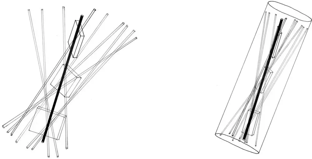
This means that we can cover ETρ=⋃T∈TρTTρ by a set of (mostly) disjoint rectangular prisms of dimensions δ/ρ×c×c, each of which have large intersection with ETρ, in the sense that ∣G∩ETρ∣≳∣G∣, for each such prism G; see Figure 2 (left).
Undoing the anisotropic rescaling associated to Tρ that was described above, we have that ⋃T[Tρ]T can be covered by a set of (mostly) disjoint rectangular prisms of dimensions δ×ρc×c;
The image shows two 3D geometric scenes. On the left, a thick black line segment is surrounded by several colored (red, green, blue) rectangular bounding boxes and numerous thin line segments. On the right, the same scene is enclosed within a transparent cylinder. The black line segment and its bounding boxes are still present, and the colored line segments are also shown within the cylinder.
The diagram illustrates a 3D geometric scene. On the left, a thick black line segment is shown with several colored (red, green, blue) rectangular bounding boxes and numerous thin line segments. On the right, the same scene is enclosed within a transparent cylinder. The black line segment and its bounding boxes are still present, and the colored line segments are also shown within the cylinder.
Scientific illustration: Geometric line segments and bounding boxes inside a 3D space and a cylinder.
Figure 2: Left: The set of tubes TTρ and the grains {G}. For clarity, we have only drawn the grains and tubes that intersect the black tube (and even most of these have been omitted; the set of red tubes passing through the red grain fill out a substantial portion of the red grain, and similarly for the other grains); the situation is similar for each tube in TTρ.
Right: The image of Figure 2 (left) after undoing the anisotropic rescaling associated to Tρ. The dimensions of each grain have changed from δ/ρ×c×c to δ×ρc×c.
see Figure 2 (right). The same statement is true for each Tρ∈Tρ. Let P denote the set of all such δ×ρc×c prisms, from all ρ tubes in Tρ. In order to bound μcoarse, it suffices to bound the typical intersection multiplicity of the prisms in P.
A coarse-scale estimate Step 2: intersection multiplicity of the grains.
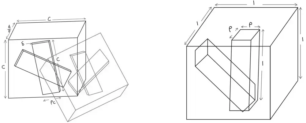
Each δ×ρc×c prism in P has an associated tangent plane, which is well-defined up to accuracy δ/(ρc). Suppose that the prisms in P intersect “tangentially,” in the sense that whenever two prisms P,P′∈P intersect, their corresponding tangent planes agree up to accuracy δ/(ρc). We will call this Simplifying Assumption C. This means that for each point x, the set of prisms from P containing x are contained in a common prism of dimensions roughly δ/ρ×c×c. Thus we can partition P into sets, P=⋃Pi, with the property that if two prisms intersect then they are contained in a common set, and the δ×ρc×c prisms in each set Pi are contained in a common prism □i of dimensions roughly δ/ρ×c×c; see Figure 3 (left).
Fix a set P′ from the partition of P described above, and let □ be the associated δ/ρ×c×c prism. The image of each P∈P′ under the anisotropic rescaling sending □ to the unit cube will be a prism of dimensions roughly ρ×ρ×1 (see Figure 3 (right)). Since a ρ×ρ×1 prism is comparable to a ρ tube, we will abuse notation slightly and pretend that this set of prisms is actually a set of ρ tubes; we will call this set T~. Our task of estimating μcoarse now reduces to estimating the typical intersection multiplicity of the tubes in T~.
A priori, we do not know anything about the structure of the set T~. A key new idea of our paper
The image contains two 3D geometric diagrams. The left diagram shows a blue cube with side length C and a red rectangular prism. The blue prism has a height of pδ and a width of δ. The red prism has a width of C and a height of pc. The right diagram shows a blue cube with side length 1 and a red rectangular prism with a width of p and a height of 1.
The left diagram illustrates a 3D space with a blue cube of side length C and a red rectangular prism. The blue prism has a height of pδ and a width of δ. The red prism has a width of C and a height of pc.
The right diagram illustrates a 3D space with a blue cube of side length 1 and a red rectangular prism. The red prism has a width of p and a height of 1.
Scientific illustration: Geometric diagrams of 3D bounding boxes and a cube with a rectangular prism.
Figure 3: Left: two sets of δ×ρc×c prisms from the partition of P (blue and red, respectively), and the associated δ/ρ×c×c prisms □ and □ that contain them.
Right: The anisotropic rescaling that maps the blue δ/ρ×c×c prism □ to the unit cube maps each blue δ×ρc×c prism to a ρ×ρ×1 prism (this is comparable to a ρ tube).
is a structure theorem that finds a set W of convex sets such that W obeys (a suitable analogue of) the Katz-Tao Convex Wolff Axioms with error ≲1, and for each W∈W, the set
T~[W]={T~∈T~:T~⊂W}
satisfies the following key properties:
1. The cardinality estimate #T~[W]≈CKT−CW(T~)⋅∣W∣/∣T~∣ (here ∣T~∣∼ρ2 denotes the volume of a tube from T~).
2. For every convex set U⊂W, we have #T~[U]≲∣W∣∣U∣#T~[W].
See Figure 5 for an illustration of this process, and Proposition 4.6 for a precise statement.
Let's analyze a special case to see what these two properties mean. Suppose for a moment that W is a τ tube for some ρ<τ<1, then Item 1 says that after rescaling W to a unit cube, T~[W] becomes a set of ρ/τ-tubes of cardinality ≳CKT−CW(T~)(τ/ρ)2. Item 2 is a non-concentration condition on these tubes that was first introduced in [26]; families of tubes obeying this non-concentration condition are said to satisfy the Frostman Convex Wolff Axioms. For example, Items 1 and 2 are satisfied if the following holds: in each ρ/τ-separated direction, we have roughly CKT−CW(T~) many parallel ρ/τ-tubes. This type of tube arrangement was previously considered by Wolff [29], and volume estimates for unions of tubes satisfying these properties are called X-ray estimates. The Assertion E(σ,ω), in particular E(1/2,0), is a generalization of Wolff's X-ray estimate from [29]. As a consequence, we should expect ⋃T~[W]T~ to have a large volume if CKT−CW(T~) is substantially greater than 1. See Case 2 below for more details.
Our argument now splits into three cases.
Case 1:CKT−CW(T~)≲1. In this case, W consists of a single convex set, which is comparable to the unit ball. To simplify this proof vignette, we will suppose that T~ satisfies the Frostman Slab Wolff
Axioms with error ≲1, and thus T~ satisfies the hypothesis of Assertion D(σ,ω); this simplification can be justified using certain rescaling arguments that we will not detail here. In particular, this means that #T~≲ρ−2, and thus we can apply Assertion D(σ,ω) to obtain the desired estimate
μcoarse≲ρσ−ω(#T~)σ≲ρ−σ−ω.
Case 2:CKT−CW(T~)≫1, and each W∈W has thickness t≫δ. To handle this case, we will consider the following analogy. Suppose that T is a set of δ tubes of cardinality mδ−2, for some m≫1. Suppose furthermore that T satisfies the Katz-Tao Convex Wolff Axioms with error m, and the Frostman Slab Wolff Axioms with error ∼1. Then Assertion E(σ,ω) says that ⋃TT has volume ≳mσ/2δσ+ω, which is substantially larger than δσ+ω. We apply a similar argument to the set of tubes T~[W] to conclude that for each W∈W, the union ⋃T~[W]T~ has large volume (see also the discussion of the two properties above). Undoing the re-scaling described in the previous step (and illustrated in Figure 3), we obtain a scale δ≪τ≪δ/ρ≥ (here τ depends on t and the orientation of W with respect to □) with the property that for a typical point x∈⋃TT, the ball Bτ=B(x,τ) has a large intersection with ⋃TT. This means that we obtain an inequality of the following form:
Bτ∩(T∈T⋃T)≳CKT−CW(T~)σ/2(δ/τ)σ+ω∣Bτ∣.(1.12)
This is precisely (1.7), provided CKT−CW(T~)≥δ−2α/σ (this is what we mean by CKT−CW(T)≫1).
Next, let Tτ be a set of essentially distinct τ tubes with the property that each T∈T is contained in some tube from Tτ, and suppose that each Tτ∈Tτ contains about (#T)/(#Tτ) tubes from T. It is straightforward to compute that CF−SW(Tτ)≲1 (indeed, this is inherited from T), and that CKT−CW(Tτ)≈(#Tτ)∣Tτ∣ (this latter quantity is ≥1, since CKT−CW(T)≲1 and thus at least ∣Tτ∣−1 essentially distinct τ tubes are needed to cover the tubes in T). Applying the estimate E(σ,ω) to Tτ, we conclude that
Tτ∈Tτ⋃Tτ≳τω((#Tτ)∣Tτ∣2)σ/2≳τω+σ.
For the last inequality, we used the estimate #Tτ≳∣Tτ∣−1, which follows from the hypotheses CKT−CW(T)≲1 and #T∼δ−2. Pairing this scale-τ estimate with our previously discussed estimate (1.12) inside balls of radius τ, we obtain (1.5):
Case 3:CKT−CW(T~)≫1, and each W∈W has thickness ≈δ. In this case, the grains in P can be replaced by larger prisms—these are the (rescaled) convex sets coming from W. This process may change ρ and also change the dimensions of the grains. We iterate the argument described above with our new ρ and larger grains. If we repeatedly find ourselves in Case 3 with each iteration, then the grains become wider and wider. Suppose for the moment that after a sufficient number of iterations, both ρ and c have size ≈1. Then ⋃TT is organized into a union of δ×1×1-slabs. From here, a straightforward geometric argument (analogous to Cordoba's proof of the Kakeya maximal function conjecture in the plane) shows that ∣⋃TT∣≈1. If instead c≪1, then a different Cordoba
type geometric argument and the assumption that μ≫1 (if this assumption fails, then we are done) allows us to enlarge c, and we iterate the argument again.
Justifying the simplifying assumptions.
We will briefly justify Simplifying Assumptions A – C. First, if Simplifying Assumption A fails, then we can directly prove (1.5) by using the sticky Kakeya theorem; see Section 10 for details. In general, Simplifying Assumption B might not hold, but if it fails, then either it is possible to directly prove (1.5), or else it is possible to find an intermediate scale between δ and ρ at which the assumption holds; this introduces additional steps and complexity to the argument, but does not fundamentally change the flavor of the proof.
If Simplifying Assumption C fails, then we can use a straightforward Cordoba-type geometric argument to show that for a typical prism P0∈P, the union of prisms P∈P that intersect P0 fill out (most of) a thickened neighbourhood of P0. This in turn means that for a typical tube T0∈T, the union ⋃TT fills out (most of) a thickened neighbourhood of T0. We can then argue as in Case 2 (described above) to obtain (1.6).
In the table below, we summarize some of the geometric objects that appeared in the arguments from Section 1.5.
object
cardinality
dimensions
bounding box
union size
desired union size
multiplicity
desired multiplicity
T
δ−2
δ×δ×1
1×1×1
≳δσ+ω
≳δσ+ω−α
≲δ−σ−ω
≲δ−σ−ω+α
T[Tρ]
δν(δ/ρ)−2
δ×δ×1
ρ×ρ×1
≲δνσ(ρδ)−σ−ω
P
δ×cρ×c
ρδ×c×c (if tangential)
μcoarse
≲ρ−σ−ω
T~
ρ×ρ×1
1×1×1
μcoarse
≲ρ−σ−ω
1.6 Tube doubling and Keleti's line segment extension conjecture
In this section we will discuss further consequences of Theorem 1.9. We begin by introducing the Tube Doubling Conjecture (see e.g. [10, Conjecture 15.19]). In what follows, if T is a δ tube in Rn, then T~ denotes the 2-fold dilate of T. Besicovitch constructed a set T of roughly δ−1 tubes in R2 for which
T∈T⋃T~≳loglog(1/δ)log(1/δ)T∈T⋃T.(1.13)
This construction was adapted by Fefferman [8] to show that the ball multiplier is unbounded on Lp for p=2. The Tube Doubling Conjecture asserts that up to sub-polynomial factors, Inequality (1.13) is tight. One formulation is as follows.
Conjecture 1.11.Let n≥2 and ε>0. Then the following is true for all δ>0 sufficiently small. Let T be a set of δ tubes in Rn. Then
T∈T⋃T~≤δ−εT∈T⋃T.(1.14)
Conjecture 1.11 is known in dimension two, and open in three and higher dimensions. As a consequence of Theorem 1.9, we resolve Conjecture 1.11 in R3.
Theorem 1.12.The Tube Doubling Conjecture is true in R3.
We will discuss the proof of Theorem 1.12 in Section 12. The Tube Doubling Conjecture is closely related to Keleti’s Line Segment Extension Conjecture [22]. In the statement that follows, if ℓ is a line segment (by definition, line segments have positive length), then ℓ~ denotes the line containing ℓ.
Conjecture 1.13.Let L be a set of line segments in Rn. Then
dim(ℓ∈L⋃ℓ~)=dim(ℓ∈L⋃ℓ).
In [23], Keleti and Máthé proved that the Kakeya set conjecture in Rn implies Conjecture 1.13 in Rn. As a consequence, Theorem 1.1 has the following corollary.
Theorem 1.14.Conjecture 1.13 is true in R3.
1.7 Thanks
The authors would like to thank Ciprian Demeter, Larry Guth, Nets Katz, Izabella Laba, Tuomas Orponen, Keith Rogers, Pablo Shmerkin, and Terence Tao for comments, suggestions, and corrections to an earlier version of this manuscript. Hong Wang would like to thank Guido de Philippis for interesting conversations. Hong Wang is supported by NSF CAREER DMS-2238818 and NSF DMS-2055544. Joshua Zahl is supported by a NSERC Discovery Grant and a NSERC Alliance Grant.
2 A sketch of the proof
Our goal in this section is to briefly outline the major steps in the proofs of Propositions 1.6 and 1.7. To simplify the exposition in this proof sketch, we will gloss over many technical details and make a number of white lies. For example, we will pretend that every shading Y(T)⊂T is just the trivial shading Y(T)=T. At the same time, we will pretend that each point x∈⋃T∈TT is always contained in the same number of tubes from T, and similarly for other collections of tubes, rectangular prisms, etc. In the same spirit as in Section 1.5, we will disregard factors of the form δε or δ−ε, and we will (somewhat informally) write A≲B to mean that A≤Cδ−εB, for some constant C that is independent of δ and some small parameter ε>0 that we will ignore for the purposes of this sketch (in Section 3 we will give a precise definition of the relation ≲, which will be used for the remainder of the proof). In the actual proof there are myriad parameters (of which ε is an example), and navigating the precise interplay between these parameters is a major technical challenge in the paper. This issue will be entirely ignored in the proof sketch.
Finally, in this proof sketch it will be helpful to introduce “informal versions” of certain definitions and theorems that occur later in the paper. These informal versions are intentionally imprecise, and often are not literally true. These informal statements will be superseded by their formal counterparts that occur later in the paper. With these caveats, we now proceed as follows.
2.1 Proposition 1.6: Assertions D and E are equivalent
Our first goal is to prove Proposition 1.6. To do this, we will iterate the following lemma:
Lemma 6.4, informal version.Let 0<ω<ω′, and suppose that both D(σ,ω) and E(σ,ω′) are true. Then E(σ,ω′−α) is true, where α>0 depends only on the quantities ω and ω′−ω.
To prove Proposition 1.6, we fix ω and σ and suppose that D(σ,ω) is true. The statement E(σ,2) is trivially true, since the volume of ⋃TT is bounded below by the volume of a single tube. We then iterate Lemma 6.4 multiple times to conclude that E(σ,ω+ε) is true for every ε>0, and thus E(σ,ω) is true.
The idea behind Lemma 6.4 is as follows. Given a set T of δ tubes, our goal is to establish the estimate
with m=CKT−CW(T) and ℓ=CF−SW(T). For simplicity we will pretend that every collection of tubes always satisfies CF−SW(T)≲1. Removing this assumption introduces a few additional difficulties that we will not discuss here.
If CKT−CW(T)≲1, then T satisfies the hypotheses of D(σ,ω), and thus we can apply the estimate D(σ,ω) to T and immediately obtain (2.1). Suppose instead that CKT−CW(T)=m≫1. This means that there is a convex set W that contains at least m∣W∣δ−2 tubes from T. The convex set W must have diameter ≥1 (since it contains at least one tube), and wlog we can suppose that it has diameter ∼1 (since the tubes in T are contained in the unit ball). Thus we may suppose that W is comparable to a rectangular prism of dimensions a×b×1, for some δ≤a≤b≤1. We will focus on the most interesting case, which is when a and b have similar size, i.e. W is comparable to a ρ tube for some δ≤ρ≤1.
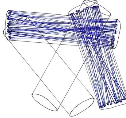
Motivated by the above discussion, let us explore what happens when CKT−CW(T)=m≫1; there is a scale δ≪ρ≪1; and a set Tρ of ρ tubes, each of which contains about m(ρ/δ)2 tubes from T. It is straightforward to verify that CKT−CW(Tρ)=O(1): if a convex set W contains N tubes from Tρ, then it contains about Nm(ρ/δ)2 tubes from T. On the other hand, W can contain at most m∣W∣/δ2 tubes from T; see Figure 4. Note that this situation is in some sense the opposite of the problematic situation described in Section 1.1 (and illustrated in Figure 1 (right)); in that Section, we considered the scenario where there are many (i.e. far more than ρ−2) ρ tubes, each of which contains few (i.e. far fewer than (ρ/δ)2) δ tubes.
We have just shown that Tρ satisfies the hypotheses of D(σ,ω), and thus
(In the above, we write ∣Tρ∣∼ρ2 to denote the volume of a ρ tube). On the other hand, for each Tρ∈Tρ, the (re-scaled) δ tubes inside Tρ will satisfy the Katz-Tao Convex Wolff Axioms with error about m, i.e. CKT−CW(TTρ)≲m=CKT−CW(T).
Applying the estimate (1.3) from Assertion E(σ,ω′), we conclude that
Inequality (2.2) says that about ρ−3+ω(#Tρ)∣Tρ∣((#T)ρ∣Tρ∣1/2)−σ distinct ρ balls are needed to cover ⋃TT, and the RHS of (2.3) gives a lower bound for the density of ⋃TT inside a typical
A 3D geometric diagram showing three cylinders. Two of the cylinders are filled with a dense network of blue lines connecting points on their surfaces. The third cylinder is empty, showing only its outline. The cylinders are arranged in a way that they intersect or are close to each other.
Scientific illustration: Geometric illustration of intersecting cylinders with blue lines connecting points.
Figure 4: Tρ (black), and T (blue). For clarity, we have only drawn the tubes from T inside two ρ tubes. Note that the ρ tubes are (comparatively) sparse, while the tubes in T[Tρ] are densely packed. The situation is similar to that in Figure 1 (left), except that the set of (rescaled) δ tubes inside each ρ tube are very dense, and thus CKT−CW(TTρ) is large.
ρ ball from this collection. Combining these estimates and noting that (#Tρ)(#T[Tρ])=#T and ∣Tρ∣∣TTρ∣=∣T∣, we conclude that
If ρ<δζ for some ζ>0 bounded away from 0, then (2.4) is precisely (2.1), with α=ζ(ω′−ω).
This concludes the proof of Lemma 6.4 and hence Proposition 1.6, except that in our proof we assumed the existence of a set of ρ tubes that satisfies the following properties:
(a) CKT−CW(Tρ)=O(1).
(b) Each ρ tube Tρ contains about m∣Tρ∣/∣T∣ tubes from T, where m=CKT−CW(T).
(c) The sets in Tρ are tubes, i.e. they have dimensions ρ×ρ×1.
(d) ρ≪1, in the sense that ρ=δζ for some ζ>0 bounded away from 0.
Unfortunately, given a set of δ tubes T, it need not be the case that such a set of ρ tubes satisfying the above properties will always exist. Consider, for example, the case where T is an arrangement of δ tubes of cardinality δ−5/2, we define s=δ5/8, and each of the roughly s−4 essentially distinct s tubes in B(0,1)⊂R3 contains one δ tube from T. Examples of this type are called the well-spaced case. For such a set T, there does not exist a scale ρ satisfying Items (a) – (d) above. Note, however, that a slightly different statement is true for this arrangement: There are scales δ≤τ≤ρ, and sets of τ and ρ tubes Tτ and Tρ that satisfy the following:
(i) T has cardinality about m∣T∣−1, where m=CKT−CW(T).
(ii) CKT−CW(Tρ)≲(#Tρ)∣Tρ∣.
(iii) Each ρ tube Tρ satisfies CKT−CW(TτTρ)=O(1), and #TτTρ∼∣TτTρ∣−1=(ρ/τ)2.
(iv) Each τ tube Tτ satisfies CKT−CW(TTτ)≲(#T[Tτ])∣TTτ∣.
(v) τ≪ρ, in the sense that τ=δζρ for some ζ>0 bounded away from 0.
For the well-spaced example described above, we would have m=δ−1/2, τ=δ, ρ=δ1/4, Tτ=T, and Tρ is a maximal set of ρ−4 essentially distinct ρ tubes.
The arguments described above can be adapted to this situation: By Item (ii), the ρ tubes satisfy the hypothesis of Assertion E(σ,ω), and thus we obtain the volume estimate
Tρ∈Tρ⋃Tρ≳ρω′(#Tρ)σ/2∣Tρ∣σ.(2.5)
Note that the RHS of (2.5) is precisely the estimate (1.3) from Assertion E(σ,ω′) (ignoring the multiplicative constant κ), with m=(#Tρ)∣Tρ∣ and ℓ=O(1).
By Item (iii), the τ tubes inside each ρ tube satisfy the hypotheses of Assertion D(σ,ω), and thus for each ρ tube Tρ we obtain the volume estimate
TτTρ∈TτTρ⋃TτTρ≳(ρτ)ω∣TτTρ∣σ/2.(2.6)
Note that the RHS of (2.6) is precisely the estimate (1.2) from Assertion D(σ,ω), with #TτTρ=∣TτTρ∣−1.
Finally, by Item (iv), the δ tubes inside each τ tube satisfy the hypothesis of Assertion E(σ,ω′), and thus for each τ tube Tτ we obtain the volume estimate
If the τ tubes are evenly distributed among ρ tubes, and the δ tubes are evenly distributed among the τ tubes, then we may suppose that for each τ tube Tτ and each ρ tube Tρ, we have (#TTτ)(#TτTρ)(#Tρ)=#T. Thus we can combine (2.5), (2.6), and (2.7) to obtain the following analogue of (2.4):
where the second equality used Item (i). By Item (v) we have τ/ρ<δζ, and thus we obtain (2.1) with α=ζ(ω′−ω), as desired.
To prove Lemma 6.4 (and hence Proposition 1.6), we show that for every arrangement of δ tubes, at least one of the following must hold.
(A) There is a set of ρ tubes satisfying Items (a) - (d) above.
(B) There are sets of τ and ρ tubes satisfying Items (i) - (v) above.
(C) The tubes in T can be efficiently packed inside rectangular prisms of dimensions s×t×1, with s≪t.
(D) The tubes in T satisfy the Frostman Convex Wolff Axioms at every scale (see Definition 6.1).
To establish the above polychotomy, in Section 4 we develop a general theory for “factoring” collections of convex sets in Rn. Given a set of δ tubes T, this allows us to find a collection of convex sets W that satisfies the analogues of Items (a) and (b) above with W in place of Tρ. If these convex sets have dimensions s×t×1 with s≪t, then this gives us Item (C). If instead s∼t, then the convex sets in W are almost tubes. We apply arguments of this type at several carefully chosen scales to show that at least one of Items (A) – (D) must hold.
The arguments described thus far establish the desired inequality (2.1) in the case where (A) or (B) holds. In Section 5 we show that Inequality (2.1) holds in Case (C); this is done using a careful rescaling argument. Finally, Case (D) is precisely the setting where we can apply the Sticky Kakeya Theorem (as generalized in [26]) to immediately conclude that T satisfies (2.1).
This concludes the proof sketch of Proposition 1.6. We now turn to Proposition 1.7.
2.2 A two-scale grains decomposition
In Sections 7 and 8, we study the structure of arrangements of δ tubes for which the estimate (1.2) from Assertion D(σ,ω) is (almost) tight, i.e. sets of δ tubes that satisfy the hypotheses of Assertion D(σ,ω), and also satisfy an inequality of the form
T∈T⋃Y(T)≲δω(#T)∣T∣((#T)∣T∣1/2)−σ.
We will assume for now that such a set T exists, and at the end of Section 2 we will arrive at a contradiction. With care, this contradiction will remain when the term δω is replaced by δω−ν for ν>0 a small positive number.
In [9], Guth proved that under mild “broadness” hypotheses, every union of δ tubes ⋃TT in R3 can be written as a disjoint union of rectangular prisms of dimensions δ×c×c, with c≥((#T)∣T∣1/2)−1; see Figure 2 (left). This lower bound on c is interesting when #T is substantially smaller than ∣T∣−1 (recall that ∣T∣ has size roughly δ2). At the opposite extreme, if #T has size about ∣T∣−1/2 (this is the smallest possible cardinality for T that is allowable, given the broadness hypotheses mentioned above), then grains have dimensions roughly δ×1×1. We remark that Guth’s methods also yield a stronger bound of the form c≥μ((#T)∣T∣1/2)−1, where μ is the number of tubes from T that pass through a typical point, but this stronger bound won’t be needed here.
First, we show that there exists a scale δ≪ρ≪1 and a set of ρ tubes Tρ so that both Tρ and the rescaled sets TTρ (recall (1.8)) satisfy the hypotheses of Assertion D(σ,ω). In addition, each rescaled set TTρ satisfies the broadness hypotheses needed to apply (a variant of) Guth’s result. Thus we can write ⋃T[Tρ]TTρ as a disjoint union of rectangular prisms of dimensions δ/ρ×c×c, where c≥((#T[Tρ])∣TTρ∣1/2)−1. Note that the grains become larger as #T[Tρ] becomes smaller; this numerology will be important later in the argument. Undoing the scaling, we obtain a partition of ⋃T[Tρ]T into disjoint δ×ρc×c rectangular prisms; we will refer to these as grains (see Figure 2 (right)), and we refer to this set of grains as GTρ. Let G=⋃TρGTρ. In our discussion below, we will call G the “two scale Guth grains decomposition” of T.
Recall that in the proof vignette outlines in Section 1.5, we made Simplifying Assumption D. We will now dicuss the technical steps needed to justify this assumption. The main goal of Section 7 is to define three “Moves,” which we will briefly describe below. After these moves have been
applied, we obtain a new scale ρ with δ≪ρ≪1; a new set of ρ tubes Tρ that cover T; and a new collection G of grains that have the following properties:
(i) Each grain has dimensions δ×ρc×c, with c≥((#T[Tρ])∣TTρ∣1/2)−1.
(ii) Each grain G∈G is associated to a unique tube Tρ∈Tρ, where G⊂Tρ, and both G and Tρ point in the same direction (up to uncertainty ρ).
(iii) Distinct grains from G associated to the same ρ tube are disjoint.
(iv) For each ρ tube Tρ, we have ⨆G=⋃T∈T[Tρ]T, where the former union is taken over the set of grains associated to Tρ.
(v) Grains associated to different ρ tubes can intersect, but this intersection must be tangential; i.e. the tangent planes of intersecting grains must agree up to uncertainty δ/(ρc).
Item (v) means that we can cover R3 by boxes of dimensions ρδ×c×c, so that each grain is contained in O(1) boxes, and two grains intersect only if they are contained in a common box. If we re-scale a box to become the unit cube, then the grains inside this box become ρ×ρ×1 rectangular prisms, i.e. ρ tubes (see Figure 2). We introduce the following notation: If □ is a ρδ×c×c box, then G□ will denote the set of ρ-tubes obtained by re-scaling the grains from G inside □. With this notation, we can state one final property for G:
(vi) For each box □, the ρ tubes in G□ satisfy the hypotheses of E(σ,ω), and CKT−CW(G□)≲1.
In a moment, we will describe the Moves needed to find a scale ρ; a set of ρ tubes Tρ; and a set of grains G that satisfy Items (i) – (vi). We begin by letting G be the two scale Guth grains decomposition of T, as described above. Items (i), (ii), (iii), and (iv) hold for this choice of G, and properties (ii)-(iv) are preserved throughout the process.
If Item (v) fails at any point in the process, then we argue by contradiction as follows. Using a L2 argument similar to Cordoba’s proof of the Kakeya maximal function conjecture in the plane, we can show that there exists some scale δ~≫δ so that the “hairbrush” of a typical grain G (i.e. the union of the grains G′∈G with G′∩G=∅) fills out (most of) the δ~-neighbourhood of G. Let us pretend that the hairbrush fills out all of the δ~ neighbourhood of G. Then for each δ tube T∈T, the corresponding δ~ tube T~=Nδ~(T) satisfies T~⊂⋃T′∈TT′. Thus we can replace our original collection of δ tubes with a new collection T~ of fatter δ~ tubes, and ⋃TT=⋃T~T~. The new collection of fatter tubes will satisfy the hypotheses of E(σ,ω) (with favorable values of CKT−CW(T~) and CF−SW(T~)), and hence we can apply the estimate E(σ,ω) to T~ and obtain a volume estimate for ∣⋃TT∣ that is superior to the estimate coming from Assertion D(σ,ω). But this contradicts the assumption that the volume estimate from Assertion D(σ,ω) was sharp for T.
We will now describe the three Moves alluded to above. For ease of exposition, it will be helpful to introduce these Moves in the opposite order that they are defined in Section 8.
Move #3 handles the situation when Item (vi) fails (recall the Assertion D(σ,ω) is sharp for T). Using an L2 argument, we show that the hairbrush of each grain G∈G fills out (most of) a wider grain G~⊃G; these wider grains have the same “length” c, but a substantially larger value of ρ. See Figure 14 for a visual depiction of this step.
Unfortunately, after applying Move #3, it might be the case that ρ has become so large that the inequality ρ≪1 is no longer true. Move #2 handles this situation. Move #2 uses a L2 argument
This demo shows the first 20 of the paper’s 127 pages. Cashmere converted all of them; the omnipub stops here to keep the demo light.
Omnipub block
Nothing selected yet.
Click any paragraph, equation, or table to see the record the omnipub keeps for it.
 Fiber
 Connect
 Omnipub
 What the PDF's own text says
 What the PDF's own text says
 1960 · English · first 20 of 36 pages
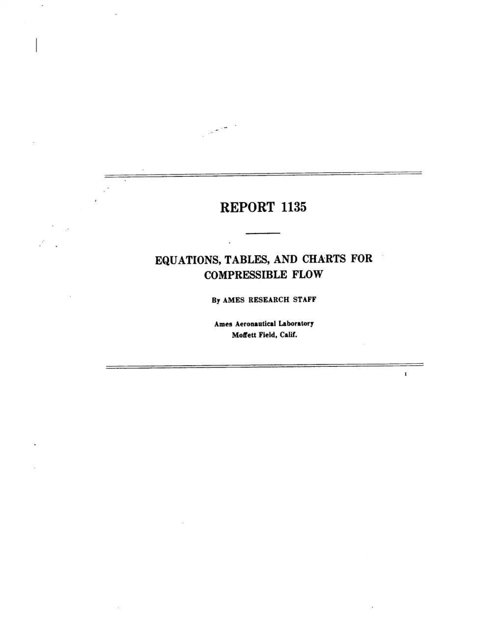 1953 · English · first 20 of 70 pages
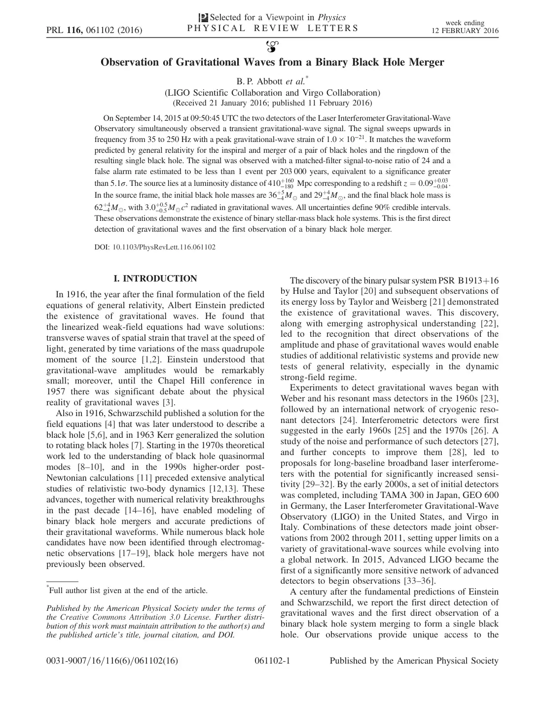 2016 · English · 16 pages
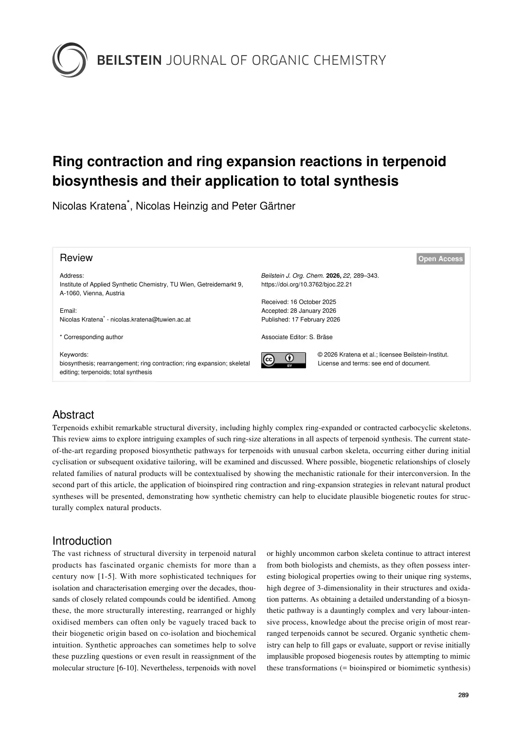 2026 · English · first 20 of 55 pages
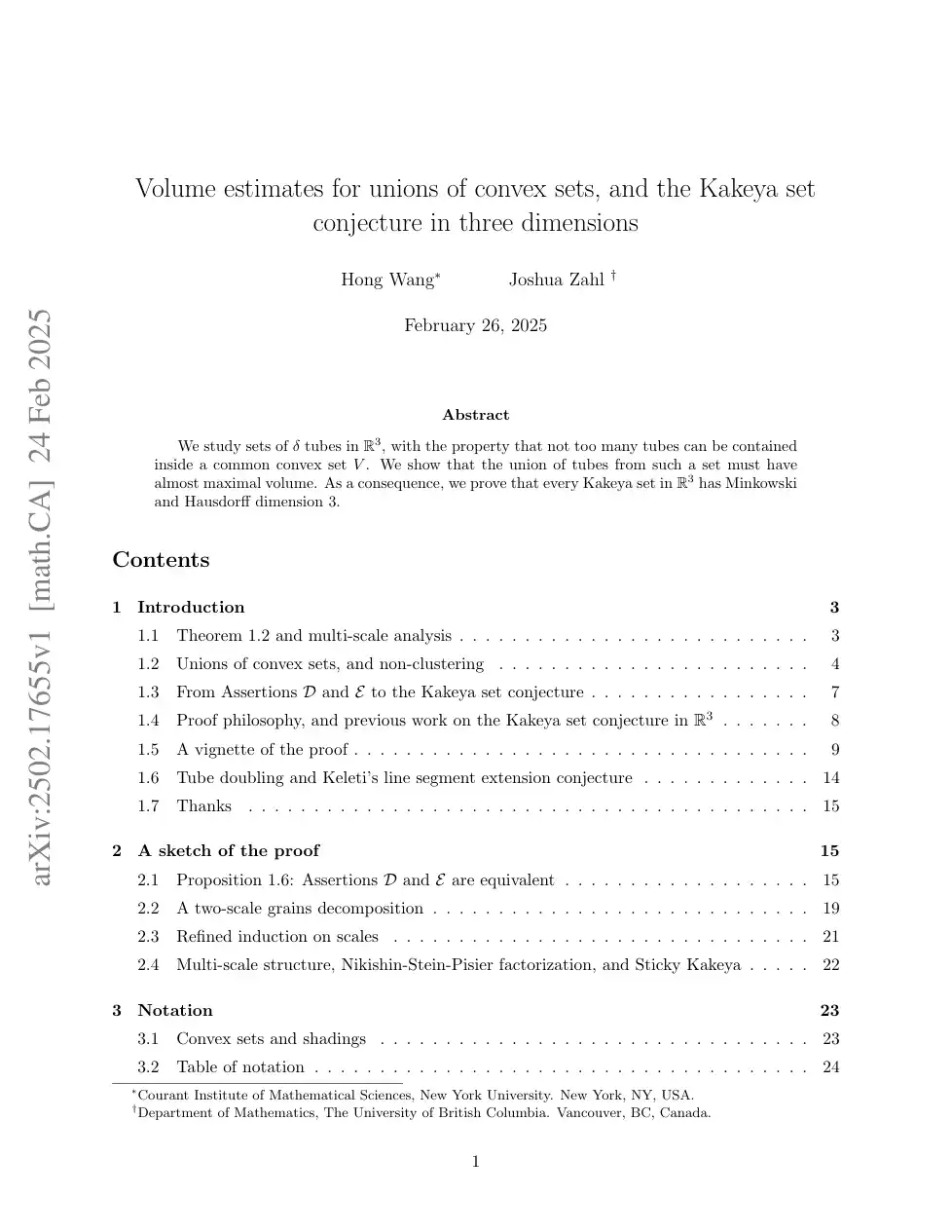 2025 · English · first 20 of 127 pages
 1905 · German · first 20 of 31 pages